Simple polarimeter
We will simulate a simple polarimeter that measures linear polarization states. In this example we will use this polarimeter to measure the polarization state of starlight.
In optical and near-infrared wavelengths it is with the current technology not possible to directly measure the electric field of starlight, only its intensity. Therefore, it is also not possible to directly measure its polarization state. However, this is a property of light that we would like to measure as it can contain important astrophysical information, e.g. on dust grain sizes and magnetic fields. To measure the polarization state we will have to encode this information into intensity measurements that, in post-processing, can be combined into an estimate of the polarization state.
We assume that the reader is familiar with basic polarization concepts, i.e. Stokes vectors, Mueller matrices, waveplates and polarizers. A good introduction on polarimetry can be found in Snik, F., & Keller, C. U. (2013). Astronomical polarimetry: polarized views of stars and planets.
In this tutorial we will use polarization optics that modulate in time to get us intensity measurements that contain polarization information. We will use a static linear polarizer, an component that only transmits one linear polarization state (e.g. horizontal polarized light), as analyzer. Before the polarizer we will put a half-wave plate (HWP). The HWP will rotate and act as the polarization modulator, which means that it transforms the linear polarization states (horizontal, vertical, +45 degree and -45 degrees) to the polarization state transmitted by the polarizer. To do so, the HWP will cycle between 0, 45, 22.5 and 67.5 degrees of rotation. For every HWP position we will measure the intensity. We can put these four intensity measurements into a vector. Multiplying this vector with the demodulation matrix results into the Stokes vector. The demodulation matrix describes how the intensity measurements encode polarization information and is based on the architecture of the polarization modulation.
As this polarimeter uses a HWP as polarization modulator, it can not transform circular polarization into the linear polarization state that the polarizer transmits. Thus this polarimeter is insenstive for circular polarization. We will see this at the end of the tutorial.
We start by importing the relevant python modules.
import numpy as np
import matplotlib.pyplot as plt

from hcipy import *
We will do our measurements with a 4 meter diameter telescope at a wavelength of 500 nanometer. This will set the spatial resolution of the system.
# parameters telescope
telescope_diameter = 4 # meter
wavelength = 500E-9 #meter

# the spatial resolution
spatial_resolution_telescope = wavelength / telescope_diameter
This allows us to set the pupil- and focal-plane grids, and the propagator.
# setting the grids
pupil_grid = make_pupil_grid(128, telescope_diameter)
focal_grid = make_focal_grid(q=6, num_airy=10, spatial_resolution=spatial_resolution_telescope)

# the propagator between the pupil- and focal-grid.
propagator = FraunhoferPropagator(pupil_grid, focal_grid)
Defining the aperture, the HWP and its positions, the linear polarizer and the detector. This detector is perfect in the sense that it has no dark current, no read noise and no flat field errors. Therefore, we will only suffer from photon noise.
aperture = make_circular_aperture(telescope_diameter)(pupil_grid)

HWP = HalfWavePlate(0)

HWP_positions = [0, 45, 22.5, 67.5] # degrees

polarizer = LinearPolarizer(0)

detector = NoisyDetector(focal_grid, dark_current_rate=0, read_noise=0, flat_field=0, include_photon_noise=False)
We now define the parameters for the starlight, e.g. its flux level and polarization state, which we eventually hope to measure.
# parameters star
zero_magnitude_flux = 3.9E10 # photons / sec
stellar_magnitude = 8

# the polarization state of the starlight.
stokes_vector_star = np.array([1,0.5,-0.01,0.05])

# Here we give the wavefront the properties (power, polarization state) of the starlight.
pupil_wavefront = Wavefront(aperture, wavelength, input_stokes_vector=stokes_vector_star)

pupil_wavefront.total_power = zero_magnitude_flux * 10**(-stellar_magnitude / 2.5)

print("Total photon flux {:g} photons / sec.".format(pupil_wavefront.total_power))
Total photon flux 2.46073e+07 photons / sec.
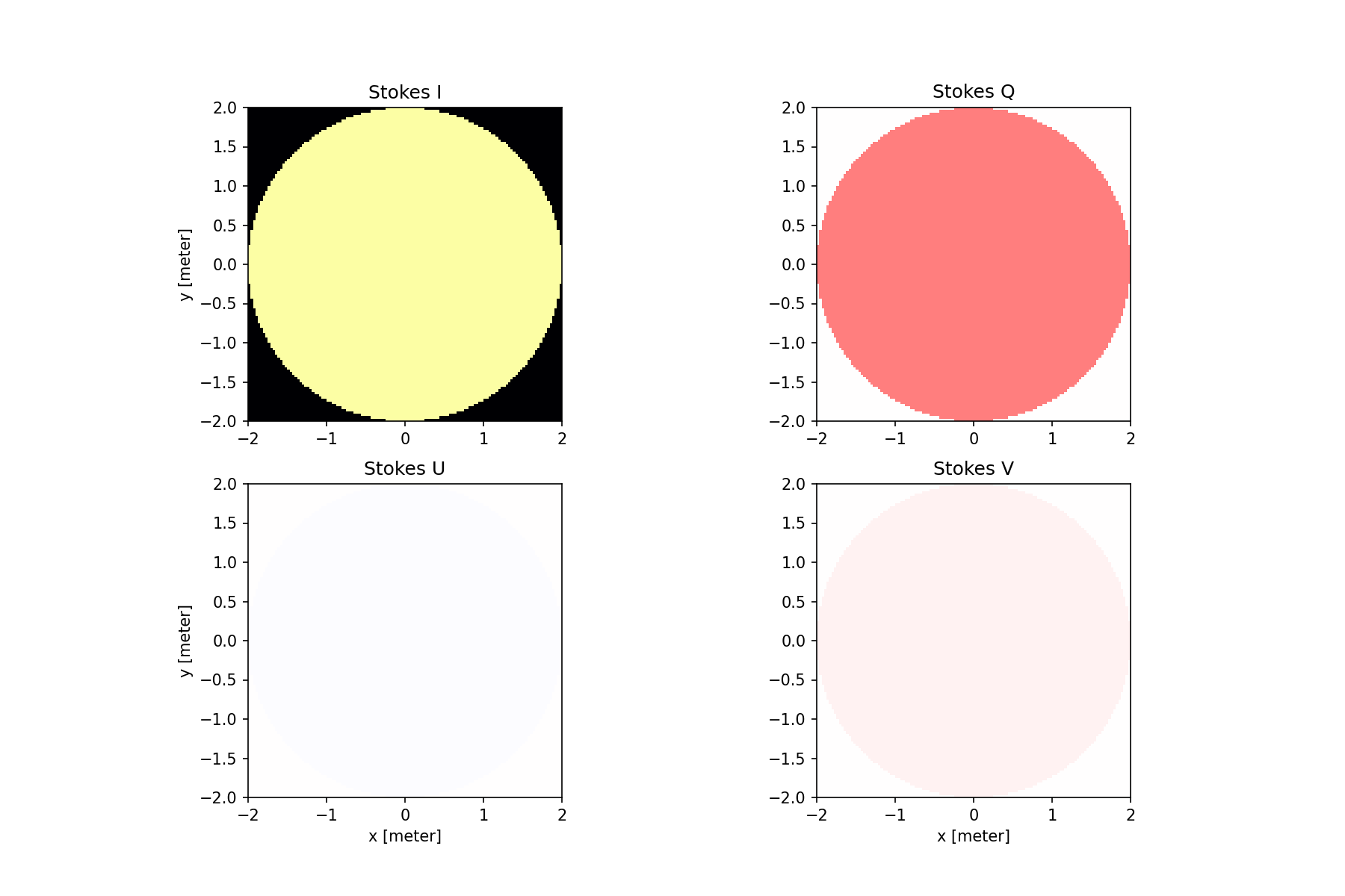
We can check the polarization state of the wavefront simply by:
stokes_parameters = [pupil_wavefront.I, pupil_wavefront.Q, pupil_wavefront.U, pupil_wavefront.V]
titles = ['I', 'Q', 'U', 'V']

# The value that we use to normalize the stokes vector with.
max_val = np.max(stokes_parameters[0])

k=1
plt.figure(figsize=(12, 8))

for stokes_parameter, title in zip(stokes_parameters, titles):
    if max_val == 0:
        max_val = 1

    plt.subplot(2,2,k)

    if title == 'I':
        cmap = 'inferno'
        vmin = 0
        vmax = 1
    else:
        cmap = 'bwr'
        vmin = -1
        vmax = 1

    if title == 'U' or title == 'V':
        plt.xlabel('x [meter]')

    if title == 'I' or title == 'U':
        plt.ylabel('y [meter]')

    imshow_field(stokes_parameter / max_val, cmap=cmap, vmin=vmin, vmax=vmax)

    plt.title('Stokes ' + title)
    k += 1
We will now simulate our polarimeter for a given time duration. During the simulation we will perform multiple HWP cycles. During one HWP cycle the HWP will rotate through its four positions. For every HWP position we will make an intensity measurement.
# total duration of the measurement
measurement_duration = 8 # seconds

# number of times we go through a HWP cycle
HWP_cycles = 4

# integration time per measurement
delta_t = measurement_duration / (HWP_cycles * 4)

# counter for the state of the modulation loop
k = 0

# The arrays where the measurements are saved
measurements = Field(np.zeros((4, focal_grid.size)), focal_grid)

# looping through the time steps
for t in np.linspace(0, measurement_duration, HWP_cycles * 4):

    # rotating the HWP to its new position
    HWP.fast_axis_orientation = np.radians(HWP_positions[k])

    # we propagate the wavefront through the half-wave plate
    pupil_wavefront_2 = HWP.forward(pupil_wavefront)

    # we propagate the wavefront through the linear polarizer
    pupil_wavefront_3 = polarizer.forward(pupil_wavefront_2)

    focal_wavefront = propagator(pupil_wavefront_3)

    detector.integrate(focal_wavefront, dt=delta_t)

    # reading out the detector in the correct element of the measurement array
    measurements[k,:] += detector.read_out()

    # Moving to the next HWP position
    k += 1

    # resetting the HWP to its intial position
    if k > 3:
        k = 0
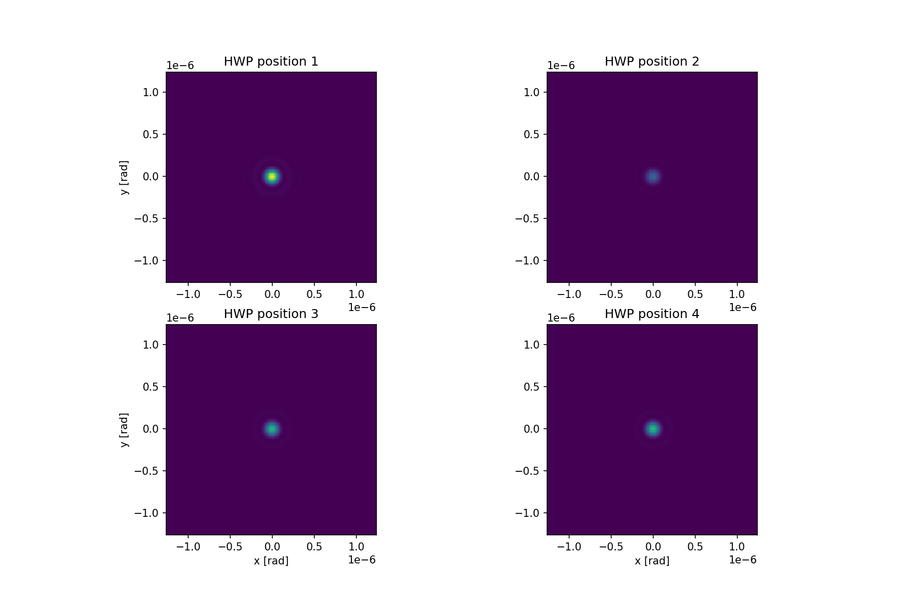
Lets plot the measurements for the various HWP positions and the total number of photons. Note that the measurements have different numbers of photons, this is due to the starlight’s polarization state.
plt.figure(figsize=(12, 8))

max_val_meas = np.max(measurements)

for i in np.arange(4):
    plt.subplot(2,2,i+1)
    imshow_field(measurements[i,:], vmin=0, vmax=max_val_meas)

    if i > 1:
        plt.xlabel('x [rad]')

    if i == 0 or i == 2:
        plt.ylabel('y [rad]')

    print('\nHWP position ', i+1)
    print('Number of photons = ', int(np.sum(measurements[i,:])))

    plt.title('HWP position ' + str(i+1))
HWP position  1
Number of photons =  36242645

HWP position  2
Number of photons =  12080881

HWP position  3
Number of photons =  23920146

HWP position  4
Number of photons =  24403381
We now have our measurements, which we want to convert into a polarization state. We do this by multiplying the measurements with a demodulation matrix. This matrix combines the measurements in such a way that the polarization state is retrieved. The demodulation matrix for this system is given by:
# defining the demodulation matrix
demodulation_matrix = np.zeros((4,4))

# demodulation for I
demodulation_matrix[0,:] = 0.25

# demodulation for Q
demodulation_matrix[1,0] = 0.5
demodulation_matrix[1,1] = -0.5

# demodulation for U
demodulation_matrix[2,2] = 0.5
demodulation_matrix[2,3] = -0.5

print('demodulation matrix = \n', demodulation_matrix)
demodulation matrix =
 [[ 0.25  0.25  0.25  0.25]
 [ 0.5  -0.5   0.    0.  ]
 [ 0.    0.    0.5  -0.5 ]
 [ 0.    0.    0.    0.  ]]
Let’s do aperture photometry on the star to construct a 1-dimensional measurement vector. We use an aperture with a diameter of the spatial resolution of the telescope (i.e. \(1\) \(\lambda/D\)).
After that, we calculate the polarization state by multiplying this vector with the demodulation matrix.
photometry_aperture = make_circular_aperture(spatial_resolution_telescope)(focal_grid)

# generating the measurement vector by doing aperture photometry.
measurement_vector = np.array(np.sum(measurements[:,photometry_aperture==1], axis=1))

# calculating the measured Stokes vector
stokes_measured = field_dot(demodulation_matrix, measurement_vector)

print('Measured Stokes vector = \n', stokes_measured / stokes_measured[0])

print('Input Stokes vector = \n', pupil_wavefront.input_stokes_vector)
Measured Stokes vector =
 [ 1.    0.5  -0.01  0.  ]
Input Stokes vector =
 [ 1.    0.5  -0.01  0.05]
We see that we can completely retrieve the linear polarization state, but that we are not able to measure circular polarization.
In this tutorial we have shown how to simulate a simple, and ideal polarimeter with hcipy. We have implemented a rotating HWP and linear polarizer, reconstructed the measured polarization state, and have seen that it can only measure linear polarization states. We have only discussed an ideal system without any noise source except photon noise. Using hcipy it is very easy to make these simulations more realistic by adding for example non-perfect polarization optics, atmospheric turbulence and adaptive optics, and detector noise (e.g. dark current, read noise, flat field effects). It is also possible to simulate polarimeters that measure all Stokes vector elements.