II - Wavefronts and optical systems

First let’s import HCIPy, and a few supporting libraries:

from hcipy import *
import numpy as np
import matplotlib.pyplot as plt

%matplotlib inline

Wavefronts in HCIPy are monochromatic. They consist of an electric field (as an HCIP Field), and a wavelength. If broadband images are needed, multiple Wavefronts must be constructed and propagated through the optical system, sampling the required wavelength range. Let us construct a Wavefront.

pupil_grid = make_pupil_grid(1024)
aperture = circular_aperture(1)(pupil_grid)

wavefront = Wavefront(aperture, 1)

A note must be made at this point regarding units. HCIPy is averse w.r.t. the used units. If the user fills in all quantities in SI, then all calculations in HCIPy will be returned in SI units. This allows the user to use any unit he/she wants, while still being able to seamlessly use dimensionless quantities. Ie. the convention that is used in this document, is that if the diameter of the aperture is 1, the wavelength is 1, and the focal length is 1 as well, then the focal-plane will be given in \(\lambda/D\).

To propagate this wavefront to the focal plane, we first need to construct a grid on which the focal plane will be sampled:

focal_grid = make_focal_grid(8, 16)

This constructs a Grid with 8 samples per \(\lambda/D\) and a 16 \(\lambda/D\) radius field of view (so 32 \(\lambda/D\) diameter field of view). Now we can construct a Fraunhofer propagator that can actually propagate the light to the focal plane.

prop = FraunhoferPropagator(pupil_grid, focal_grid)

img = prop.forward(wavefront)

imshow_field(np.log10(img.intensity / img.intensity.max()), vmin=-5)
plt.colorbar()
plt.show()

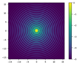
All Fourier transforms concerning the propagation are done internally. In this case a Matrix Fourier transform was used, as it was deemed quicker than a Fast Fourier transform in this case. Also note that when defining the propagator, we didn’t pass the wavelength of the wavefront. This wavelength is taken from the Wavefront object during the propagation.

Also note that a Wavefront supports many properties to make it easier to use. One that we used above is Wavefront.intensity, but others exist as well: for example Wavefront.phase and Wavefront.amplitude, which yield the phase and amplitude of the electric field respectively. All these properties are returned as Fields, and can therefore be shown using imshow_field().

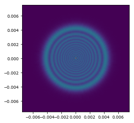
For a more interesting results, let’s do a propagation with physical quantities. We calculate the intensity pattern of a circular aperture with a diameter of 1cm, after a free-space propagation of 2m, at a wavelength of 500nm.

pupil_grid_2 = make_pupil_grid(1024, 0.015)
aperture_2 = circular_aperture(0.01)(pupil_grid_2)

fresnel_prop = FresnelPropagator(pupil_grid_2, 2)

wf = Wavefront(aperture_2, 500e-9)
img = fresnel_prop(wf)

imshow_field(img.intensity)
plt.show()

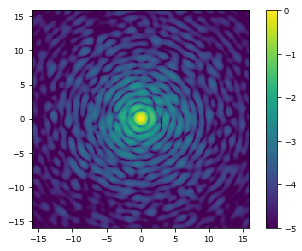
The propagators shown previously are part of a larger group of optical elements. All OpticalElements can propagate a Wavefront through them. Examples include simple Apodizers, which act as an infinitely-thin screen with a (complex) transmission. A little more complicated example is SurfaceAberration, which simulates a surface error with a power-law PSD (power spectral density). Optical elements can be linked to represent more complicated optical systems.

aberration = SurfaceAberration(pupil_grid, 0.25, 1)

wf = Wavefront(aperture)
img = prop(aberration(wf))

imshow_field(np.log10(img.intensity / img.intensity.max()), vmin=-5)
plt.colorbar()
plt.show()

c:\users\emiel por\documents\github\hcipy\hcipy\optics\aberration.py:39: RuntimeWarning: divide by zero encountered in power
  res = Field(grid.as_('polar').r**exponent, grid)

These simple optical elements can be combined into more complicated optical systems. These include full wavefront sensor implementations and coronagraphs. Both of these will be handled in later sections.

To convert a Wavefront into an observed image, one can simply use the Wavefront.power attribute, which is the Wavefront.intensity multiplied by the weight at each pixel. If one wants to use a more complicated detector model, HCIPy supplies a Detector class. and its derivatives. A detector uses an integration/readout scheme:

flat_field = 0.01
dark = 10
detector = NoisyDetector(focal_grid, dark_current_rate=dark, flat_field=flat_field)

wf.total_power = 5000
img = prop(aberration(wf))

detector.integrate(img, 0.5)
image = detector.read_out()

imshow_field(np.log10(image), vmax=np.log10(image).max(), vmin=0)
plt.colorbar()
plt.show()

C:\ProgramData\Anaconda3\lib\site-packages\ipykernel_launcher.py:11: RuntimeWarning: divide by zero encountered in log10
  # This is added back by InteractiveShellApp.init_path()