Making a broadband telescope point spread function
We will introduce the basic elements in HCIPy and produce a broadband point spread function for the Magellan telescope.
import numpy as np
import matplotlib.pyplot as plt

from hcipy import *
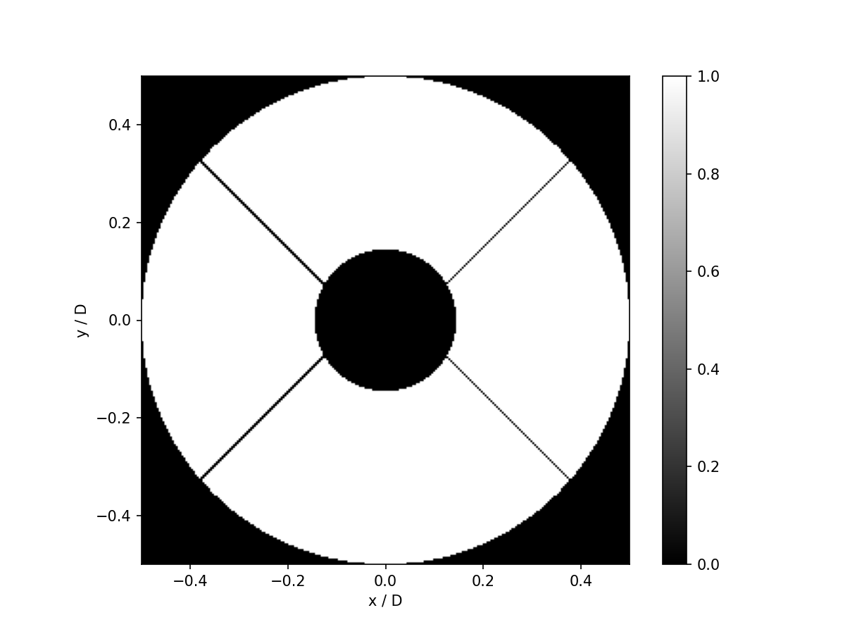
We’ll start by making a telescope pupil, then explain the code below.
pupil_grid = make_pupil_grid(256)

telescope_pupil_generator = make_magellan_aperture(normalized=True)

telescope_pupil = telescope_pupil_generator(pupil_grid)

im = imshow_field(telescope_pupil, cmap='gray')
plt.colorbar()
plt.xlabel('x / D')
plt.ylabel('y / D')
plt.show()
A lot happened in these few lines. Let’s break it down.
We first made a grid, specifically a pupil grid. A Grid defines the
sampling in some space, in essence providing the positions in \(x\)
and \(y\) for each pixel in the telescope pupil. A Grid consists
of Coords, which provide a list of coordinates, and a coordinate
system, that tells the Grid how to interpret these numbers, for
example cartesian or polar. You can also think of a Grid as
a mapping between a one-dimensional index and a corresponding position
in space.
The function make_pupil_grid() did two things. It made Coords
object with regularly-spaced coordinates, then made a CartesianGrid
object out of them. A pupil grid will always be symmetric around the
origin, and will be
Finally, a Field is a combination of a one-dimensional array of
numbers with an associated Grid. A Field can be thought of as a
sampled physical field, such as temperature, potential, electric field,
intensity, etc… Many functions in HCIPy use Fields to correctly
handle their sampling requirements. For example, when plotting a
Field, you do not have to supply an extent, as that is already given
by the Field itself. Another example is a Fast Fourier Transform
(FFT). Taking an FFT of a Field will return a Field for which
its Grid is in frequency units. Scaling the Grid of the input
Field will correspondingly change the Grid of the returned
Field. As HCIPy keeps track of the sampling throughout your code, it
makes it extremely hard to introduce human errors in sampling.
So how do we now make a Field object? We can of course manually
supply the values for each pixel, but here we take an easier approach.
There are many Field generators in HCIPy. These are functions that
can be evaluated on a Grid. Here we create a Field generator
using make_magellan_aperture(), which returns the telescope pupil
for the Magellan 6.5m
telescope at Las Campanas
Observatory in Chile. You can think of Field generators as a
mathematical description of some function, which can be sampled on a
Grid by evaluating it.
The next line evaluates the telescope pupil on our previously generated
Grid. The last few lines then display the Field as an image
using the function imshow_field(). This function mimics the standard
pyplot.imshow() in matplotlib, and they can be largely
considered interchangeable. Note that imshow_field() used the
Grid of the telescope aperture and correctly displays the numbers on
the axes.
Now that we have a telescope pupil, we can start creating the point spread function (PSF) for the telescope. Again, we’ll explain the code below.
wavefront = Wavefront(telescope_pupil)

focal_grid = make_focal_grid(q=8, num_airy=16)
prop = FraunhoferPropagator(pupil_grid, focal_grid)

focal_image = prop.forward(wavefront)

imshow_field(np.log10(focal_image.intensity / focal_image.intensity.max()), vmin=-5)
plt.xlabel('Focal plane distance [$\lambda/D$]')
plt.ylabel('Focal plane distance [$\lambda/D$]')
plt.colorbar()
plt.show()
<>:9: SyntaxWarning: "l" is an invalid escape sequence. Such sequences will not work in the future. Did you mean "\l"? A raw string is also an option.
<>:10: SyntaxWarning: "l" is an invalid escape sequence. Such sequences will not work in the future. Did you mean "\l"? A raw string is also an option.
/tmp/ipykernel_2538/1921514947.py:9: SyntaxWarning: "l" is an invalid escape sequence. Such sequences will not work in the future. Did you mean "\l"? A raw string is also an option.
  plt.xlabel('Focal plane distance [$lambda/D$]')
/tmp/ipykernel_2538/1921514947.py:10: SyntaxWarning: "l" is an invalid escape sequence. Such sequences will not work in the future. Did you mean "\l"? A raw string is also an option.
  plt.ylabel('Focal plane distance [$lambda/D$]')
We want to see what happens when we image a point source (such as a
distant star) with a telescope that has this particular telescope pupil
geometry. We first create a Wavefront object, and pass it the
telescope pupil as the corresponding electric field. This Wavefront
is the light just after it reflected of the Magellan primary mirror.
Wavefronts are used for all light in HCIPy, and they can be
modified by propagating the light through OpticalElements, but
more on that below.
We now need to define the sampling of the PSF that we want to obtain.
This is done with the make_focal_grid() function. This function
takes q, which is the number of pixels per diffraction width, and
num_airy, which is half size (ie. radius) of the image in the number
of diffraction widths.
We now define our first OpticalElement. The FraunhoferPropagator
object is a propagator that simulates the propagation through a
telecentric reimaging system, from a pupil plane to a focal plane. It
requires the sampling of the input pupil and the sampling of the output
focal plane as arguments.
We can use this Propagator to propagate our Wavefront to the
focal plane of the telescope. This is done by calling the forward()
function with the Wavefront as an argument. This returns a new
Wavefront, now in the focal plane of the telescope.
Again, we use imshow_field to show the intensity of the focal-plane
image on a logarithmic scale.
Next, we want to take a cut across this image to see what how the flux
changes as a function of angular separation from the on-axis position in
units of diffraction widths \((\lambda/D)\). focal_image is a
Wavefront object, which has several properties including
intensity, so we use that:
psf = focal_image.intensity
Next we want to know the size and shape of the psf, but it’s stored
as a 1D list of values. In some cases, including now, it is still useful
to have a two-dimensional image instead. We can use the shaped
attribute to get a reshaped version of psf, which has the shape
according to its grid. We can then cut out the middle row from the image
using [:,psf_shape[0] // 2] remembering that we need to have shaped
the psf first before doing the slicing, and then we normalise the
slice by the peak value of the psf image.
psf_shape = psf.grid.shape

slicefoc = psf.shaped[:, psf_shape[0] // 2]
slicefoc_normalised = slicefoc / psf.max()
Finally we plot out the normalised slice. Note that HCIPy keeps track of
the units and coordinates so that you don’t have to propagate them
yourself and risk making an error in the process - we get the units by
taking the x values from the focal_grid, remembering to
reshape them to a 2D array, and then slicing out one of the rows and
using these values for the x axis of our plot:
plt.plot(focal_grid.x.reshape(psf_shape)[0, :], slicefoc_normalised)
plt.xlabel('Focal plane distance [$\lambda/D$]')
plt.ylabel('Normalised intensity [I]')
plt.yscale('log')
plt.title('Magellan telescope PSF in diffraction units')
plt.xlim(-10, 10)
plt.ylim(5e-6, 2)
plt.show()
<>:2: SyntaxWarning: "l" is an invalid escape sequence. Such sequences will not work in the future. Did you mean "\l"? A raw string is also an option.
<>:2: SyntaxWarning: "l" is an invalid escape sequence. Such sequences will not work in the future. Did you mean "\l"? A raw string is also an option.
/tmp/ipykernel_2538/1865244475.py:2: SyntaxWarning: "l" is an invalid escape sequence. Such sequences will not work in the future. Did you mean "\l"? A raw string is also an option.
  plt.xlabel('Focal plane distance [$lambda/D$]')
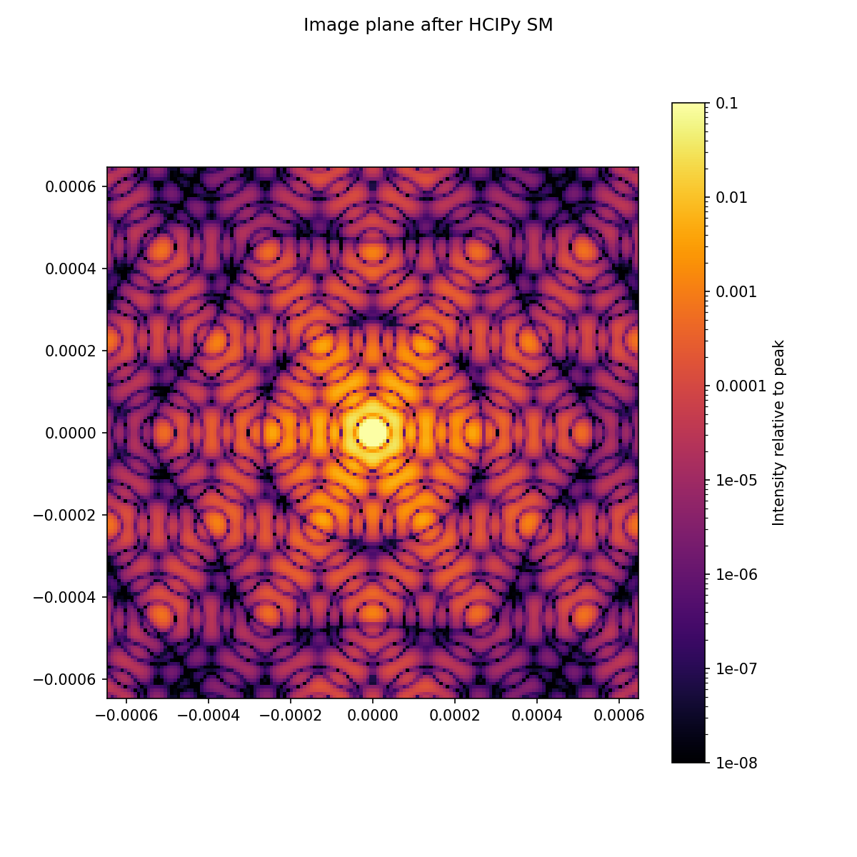
We’ve plotted up the monochromatic case, but now let’s see the effect
for broadening the range of wavelengths through our telescope - we
adjust the wavelength in the wavefront, then calculate the intensity
image and add them together for several different wavelengths. We pick
11 monochromatic PSFs over the fractional bandwidth:
bandwidth = 0.2

focal_total = 0
for wlen in np.linspace(1 - bandwidth / 2., 1 + bandwidth / 2., 11):
    wavefront = Wavefront(telescope_pupil, wlen)
    focal_total += prop(wavefront).intensity

imshow_field(np.log10(focal_total / focal_total.max()), vmin=-5)

plt.title('Magellan PSF with a bandwidth of {:.1f} %'.format(bandwidth * 100))
plt.colorbar()
plt.xlabel('Focal plane distance [$\lambda/D$]')
plt.ylabel('Focal plane distance [$\lambda/D$]')
plt.show()
<>:12: SyntaxWarning: "l" is an invalid escape sequence. Such sequences will not work in the future. Did you mean "\l"? A raw string is also an option.
<>:13: SyntaxWarning: "l" is an invalid escape sequence. Such sequences will not work in the future. Did you mean "\l"? A raw string is also an option.
/tmp/ipykernel_2538/1875355710.py:12: SyntaxWarning: "l" is an invalid escape sequence. Such sequences will not work in the future. Did you mean "\l"? A raw string is also an option.
  plt.xlabel('Focal plane distance [$lambda/D$]')
/tmp/ipykernel_2538/1875355710.py:13: SyntaxWarning: "l" is an invalid escape sequence. Such sequences will not work in the future. Did you mean "\l"? A raw string is also an option.
  plt.ylabel('Focal plane distance [$lambda/D$]')
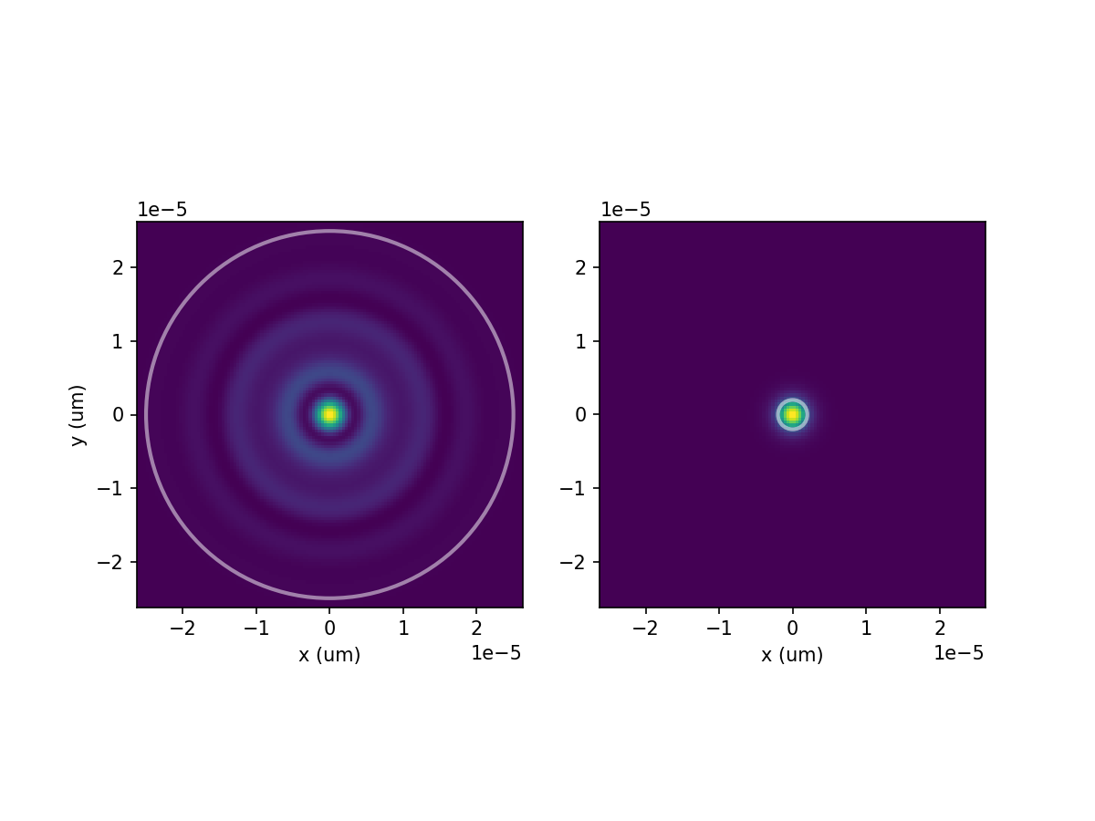
Until now, we’ve used normalized units. That is, all distances in the pupil have been in fractions of the pupil diameter, all distances in the focal plane have been in diffraction widths, the wavelength was one, and the focal length was one. While HCIPy will commonly assume normalized units as default arguments, we can also use physical units. We will now recreate the monochromatic PSF with physical units.
pupil_diameter = 6.5 # m
effective_focal_length = 71.5 # m
wavelength = 750e-9 # m

pupil_grid = make_pupil_grid(256, diameter=pupil_diameter)

telescope_pupil_generator = make_magellan_aperture()
telescope_pupil = telescope_pupil_generator(pupil_grid)

imshow_field(telescope_pupil, cmap='gray')
plt.colorbar()
plt.xlabel('x [m]')
plt.ylabel('y [m]')
plt.show()

wavefront = Wavefront(telescope_pupil, wavelength)

focal_grid = make_focal_grid(q=4, num_airy=16, pupil_diameter=pupil_diameter, focal_length=effective_focal_length, reference_wavelength=wavelength)
prop = FraunhoferPropagator(pupil_grid, focal_grid, focal_length=effective_focal_length)

focal_image = prop.forward(wavefront)

imshow_field(np.log10(focal_image.intensity / focal_image.intensity.max()), vmin=-5, grid_units=1e-6)
plt.xlabel('Focal plane distance [um]')
plt.ylabel('Focal plane distance [um]')
plt.colorbar()
plt.show()

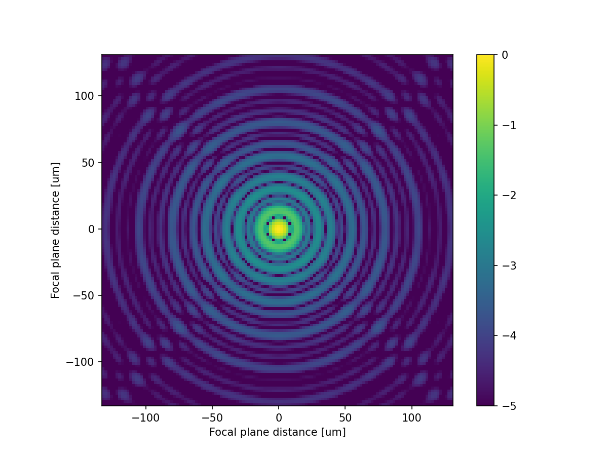
The changes from this code to that for normalized units, is that the
diameter of the telescope pupil was given to make_pupil_grid(), that
a wavelength was given to the Wavefront, that the pupil diameter,
focal length and wavelength were given to make_focal_grid() and that
the focal length was given to the FraunhoferPropagator. Also note
that we have used the parameter grid_units in the call to
imshow_field() to give the numbers on the axes in micron, instead of
meters.
The function make_focal_grid() can actually be called in many
different ways. We can either supply:
nothing, in which case normalized units are assumed;
a spatial resolution, which is the size of diffraction width;
a F-number and reference wavelength;
a pupil diameter, focal length and reference wavelength.
This allows for much flexibility in defining your sampling at the focal plane.