I - Coordinates, Grids and Fields

HCIPy is a Python library for high-contrast imaging simulations. It uses the concept of a Field to simplify syntax and avoid user error. The concept of Fields, and their corresponding Grids and Coords is an integral part of HCIPy and is used throughout the codebase. This first chapter will focus on ways to create, modify and use Fields.

First let’s import HCIPy, and a few supporting libraries:

from hcipy import *
import numpy as np
import matplotlib.pyplot as plt

%matplotlib inline

A Grid defines a set of points in space. There are many functions available for creating a Field from scratch. One of these is make_uniform_grid(). This function creates a regularly-spaced grid of points in \(N\)-dimensions in Cartesian space. The following code creates a Grid and plots the set of points using Matplotlib.

grid = make_uniform_grid([64,64], [2,1])

plt.plot(grid.x, grid.y, '+')
plt.axis('equal')
plt.xlabel('x')
plt.ylabel('y')
plt.show()

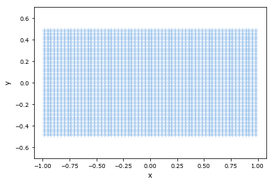
Depending on the coordinate system of the Grid, it exposes the arguments x, y, z for Cartesian coordinates, or r,theta for polar coordinates. Simply said, the Grid facilitates the conversion between an index, and a point in \(N\)-dimensional space.

The coordinate values for each dimension are stored internally in a Coords object. There exist some variants of this type of object. Each of these derived classes indicates a structure in the coordinate values. For instance, in the case above:

print('Class of grid:', grid.coords.__class__)
print('Distance between points:', grid.delta)
print('Number of points on each dimension:', grid.dims)
print('Zero-point of the grid:', grid.zero)

Class of grid: <class 'hcipy.field.coordinates.RegularCoords'>
Distance between points: [ 0.03125   0.015625]
Number of points on each dimension: [64 64]
Zero-point of the grid: [-0.984375  -0.4921875]

A RegularCoords object doesn’t store the values of each point explicitly, but rather calculates those on the fly from three parameters: 1) the distance between points, 2) the number of points on each dimension, 3) the zero point.

Let’s use another coordinate system, and differently structured coordinates. We explicitly show how a Grid is constructed.

r = np.logspace(-1, 1, 11)
theta = np.linspace(0,2*np.pi, 11, endpoint=False)
coords = SeparatedCoords((r, theta))

polar_grid = PolarGrid(coords)
cart_grid = polar_grid.as_('cartesian')

plt.plot(cart_grid.x, cart_grid.y, '+')
plt.axis('equal')
plt.show()

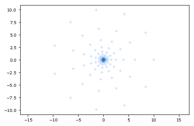
Note that to plot the points of this polar grid, we have converted the polar grid to a Cartesian grid. Accessing the Cartesian coordinates on a polar grid is not allowed:

try:
    print(polar_grid.x) # Doesn't work
except AttributeError as err:
    print(err)

'PolarGrid' object has no attribute 'x'

Each Grid also stores the weight of each point, that is, the interval, area, volume or hyper-volume that a point subtends in its space. They can be used to simplify doing integrations or taking derivatives on a Grid. In some cases, the weights can be calculated automatically, for example when the grid has regular or separated coordinates. For other coordinate structures, the weights must be supplied by the user, for example for an UnstructuredCoords.

A Field is a sampled function on a Grid. They can be though of as a physical field, sampled on each point of a Grid. We can simply construct a field by:

values = np.exp(-(grid.x**2 * 10)) * np.sin(20 * grid.y)
field = Field(values, grid)

imshow_field(field)
plt.colorbar()
plt.show()

A field can be shown by using imshow_field(), which acts very similar to the standard Matplotlib pyplot.imshow() function. It however does some things in the background. The axes are set to the correct values, according to the Grid of the Field. Additionally, it supports many other features. For instance, a complex valued field is automatically converted to a two-dimensional colorscale.

values2 = np.exp(1j * grid.x * 20) * np.sqrt(np.abs(np.sinc(5*grid.y)))
field2 = Field(values2, grid)

imshow_field(field2)
plt.show()

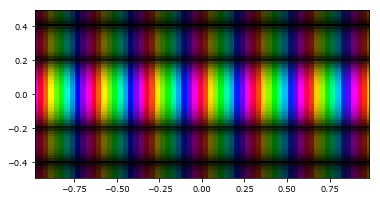
These images can be extremely useful for viewing both phase and amplitude of a complex speckle field at the same time. Additionally, it supports masking out parts of the array during plotting:

mask = circular_aperture(0.7)(grid)

imshow_field(field2, mask=mask)
plt.show()

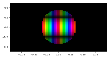
The function circular_aperture(0.7) here constructs a so-called Field generator. These are functions that take a grid as their sole parameter, and spit out a Field on that grid. Essentially, this can be used to calculate any analytical function at a set of points. Some classes and functions in HCIPy take Field generators as arguments, and they are used as output in some cases as well. An important class of Field generators are those generated by aperture functions. These include the above mentioned circular_aperture, but also rectangular_aperture, hexagon_aperture, or even complete telescopes, such as make_magellan_aperture:

pupil_grid = make_pupil_grid(128)
aperture = make_magellan_aperture(True)

imshow_field(aperture(pupil_grid), cmap='gray')
plt.show()

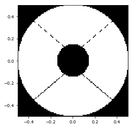
As the spiders for the Magellan aperture are very small, we have some aliasing effects. This can be avoided using supersampling during the evaluation. HCIPy implements standard functions for these:

pupil = evaluate_supersampled(aperture, pupil_grid, 8)
imshow_field(pupil, cmap='gray')
plt.show()