Design of vector-Apodizing Phase Plate patterns
This tutorial introduces the basics of designing a phase pattern for a vector-Apodizing Phase Plate (vAPP) coronagraph.
We’ll start by importing all relevant libraries and setting up our pupil and focal grids.
from hcipy import *
import numpy as np
import matplotlib.pyplot as plt
from mpl_toolkits.axes_grid1 import make_axes_locatable

pupil_grid = make_pupil_grid(512)
focal_grid = make_focal_grid(4, 20)

prop = FraunhoferPropagator(pupil_grid, focal_grid)
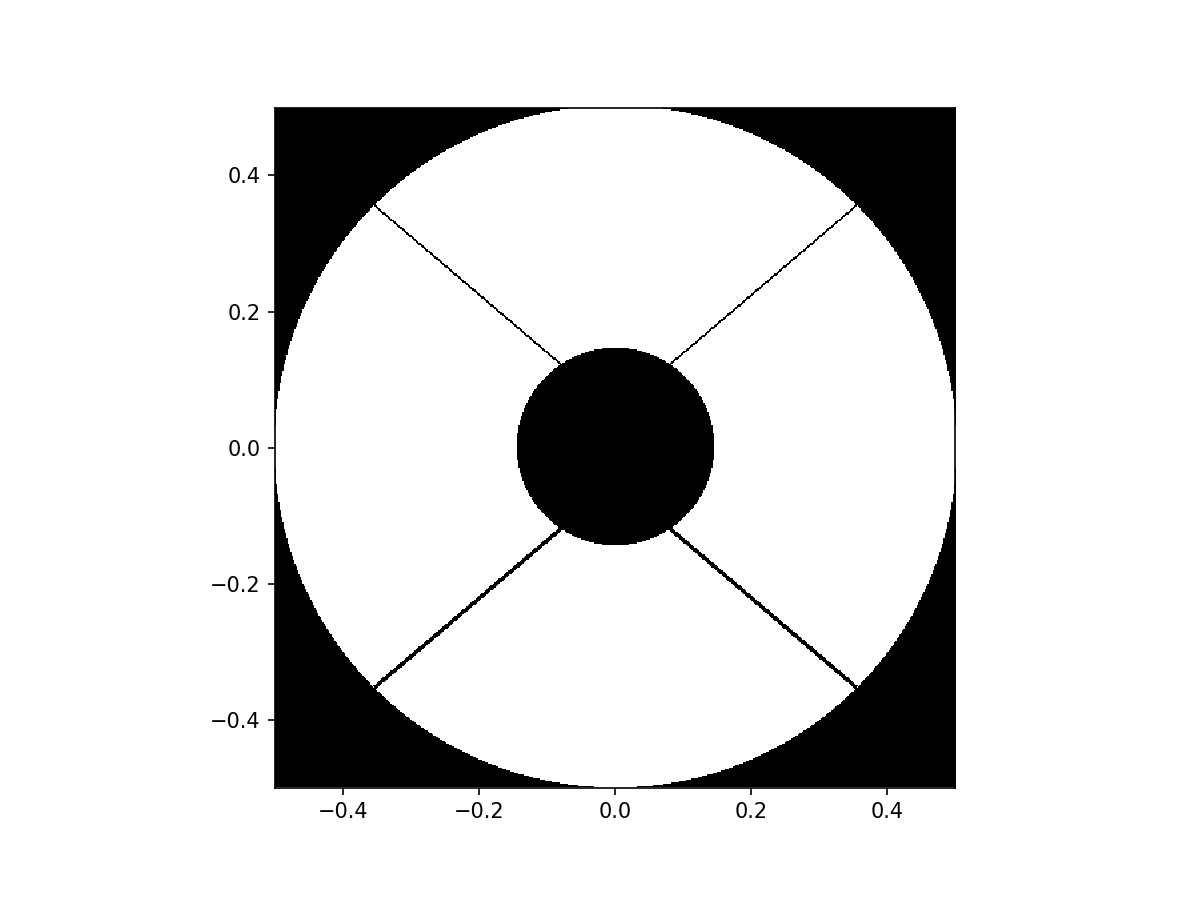
The design of the vAPP, i.e. the phase pattern, is uniquely defined by the pupil of a telescope or instrument, and the dark zone shape. Here we design a semi-realistic vAPP for the Magellan telescope using the existing make_magellan_aperture function.
aperture = make_magellan_aperture(True)

telescope_pupil = aperture(pupil_grid)

imshow_field(telescope_pupil, cmap='gray')
plt.show()
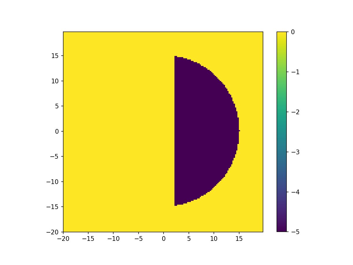
Now we are going to define the dark zone. For this tutorial, we would like the dark zone to have a ‘D’ shape and a contrast of \(10^{-5}\) relative to the stellar core.
We define the inner working angle by the separation from the star where the desired contrast level is reached and set it to of 2 \(\lambda/D\). The outer working angle is 15 \(\lambda/D\).
The dark zone is created as a pixel mask on the focal grid. From this pixel mask we create a contrast map by multiplying with the contrast level.
contrast_level = 1e-5

dark_zone = (circular_aperture(30)(focal_grid)).astype(bool)*(focal_grid.x>2)

contrast = focal_grid.ones()

contrast[dark_zone] = contrast_level

imshow_field(np.log10(contrast))
plt.colorbar()
plt.show()
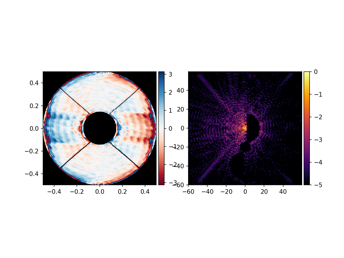
We define a plot function for the vAPP that shows the phase pattern and PSF of a vAPP.
def plot_vapp(vAPP, prop):
    '''Plot the phase pattern and PSF of a vAPP

    Parameters
    ---------
    vAPP : Wavefront
        The wavefront of a vAPP mask, containing the vAPP pattern as phase and
        the telescope pupil as amplitude
    prop : Function
        A propagator function that propagates the wavefront to a focal plane
    '''

    # Plotting the phase pattern and the PSF
    fig = plt.figure()
    ax1 = fig.add_subplot(121)
    im1 = imshow_field(vAPP.phase, mask=vAPP.amplitude, cmap='RdBu')

    divider = make_axes_locatable(ax1)
    cax = divider.append_axes('right', size='5%', pad=0.05)
    fig.colorbar(im1, cax=cax, orientation='vertical')

    ax2 = fig.add_subplot(122)
    im2 = imshow_field(np.log10(prop(vAPP).intensity/np.max(prop(vAPP).intensity)),vmin = -5, cmap='inferno')

    divider = make_axes_locatable(ax2)
    cax = divider.append_axes('right', size='5%', pad=0.05)
    fig.colorbar(im2, cax=cax, orientation='vertical')
    plt.show()
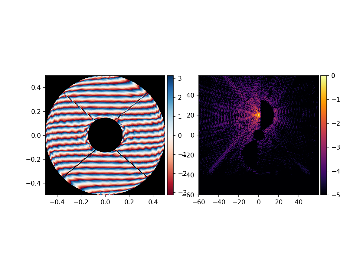
Now that everything is set up, we can start generating the vAPP phase pattern.
We use an updated version of the Gerchberg-Saxton algorithm to do the calculation. This is an iterative method, so we set the number of iterations to be 80.
We generate the input wavefront from the electric field in the pupil. Note that it is possible to use a pre-calculated wavefront that is optimized using different methods.
The output wavefront called ‘vAPP’ has unity amplitude in the pupil and the desired phase pattern of the vAPP.
# Setting up the vAPP calculation parameters.
num_iterations = 80
wavefront = Wavefront(telescope_pupil, 1)

# Generate the vAPP pattern.
vAPP = generate_app_keller(wavefront, prop, contrast, num_iterations, beta = 1)

plot_vapp(vAPP, prop)
For a classical apodizing phase plate, the design would be finished.
However, the vector-apodizing phase plate applies gemeometric phase with a sign that depends on the circular polarization state of the incoming light. This is explained in detail in the “VectorApodizingPhasePlate” tutorial.
In short, this means that without splitting the PSFs in circular polarization, the bright-side of one polarization state would be imaged on the dark zone of the orthogonal polarization state.
This has three consequences. 1. We need to separate the two polarization states by adding a phase ramp in the y-direction. This is the grating-vAPP. 2. We need to add dark zones on different locations in the focal plane to make sure that the two coronagraphic PSFs do not add light in the dark zone of the orthogonal polarization state. 3. A polarization leakage PSF, that is not apodized by the vAPP, will be imaged on the optical axis. This PSF can be used as a photometric reference if there is a dark zone for both coronagraphic PSFs there as well.
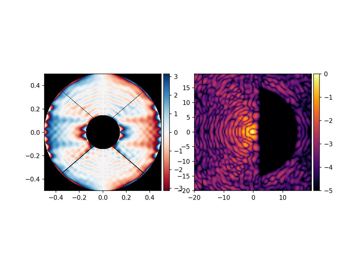
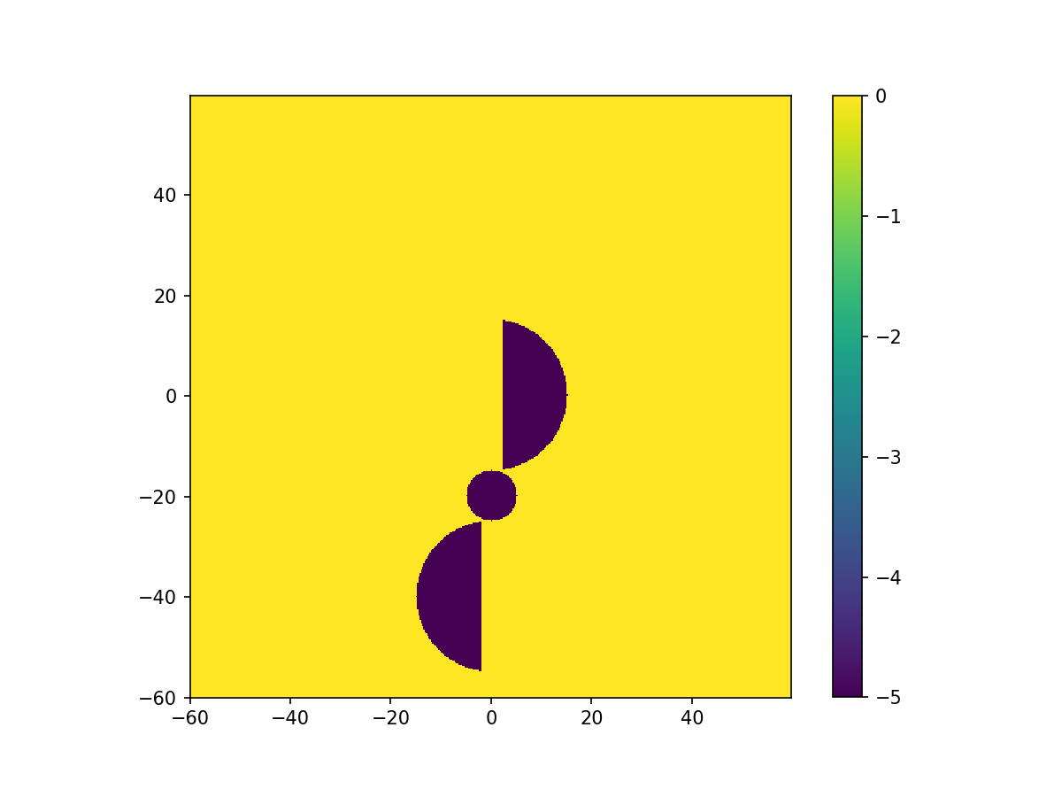
We decide that the central circular dark zone has a radius of 5 \(\lambda/D\). Combined with the 15 \(\lambda/D\) radius of the previous dark zone, we decide that we need a separation of 20 \(\lambda/D\).
Because we are adding the phase ramp to split the polarization states in a later stage, we calculate the locations of all three dark zones from the coordinate system of one coronagraphic PSF.
Therefore, we do not need to shift the D-shaped dark zone to 20 \(\lambda/D\) in the y-direction, but leave that on-axis. We shift the circular dark zone by -20 \(\lambda/D\) in the y-direction, and add a second D-shaped dark zone with flipped orientation at -40 \(\lambda/D\) in the y-direction. A larger focal grid is needed to contain the new dark zone mask.
# Updating focal grid
focal_grid_upd = make_focal_grid(4, 60)

# Generating the three dark zones
dark_zone_upd = (circular_aperture(30)(focal_grid_upd)).astype(bool)*(focal_grid_upd.x>2)
dark_zone_upd += circular_aperture(10)(focal_grid_upd.shifted((0,20))).astype(bool)
dark_zone_upd +=  (circular_aperture(30)(focal_grid_upd.shifted((0,40)))).astype(bool)*(focal_grid_upd.x<-2)

# Making the contrast map
contrast = focal_grid_upd.ones()
contrast[dark_zone_upd] = contrast_level

# Plotting the contrast map
imshow_field(np.log10(contrast))
plt.colorbar()
plt.show()
With this updated dark zone, we can calculate the phase pattern again using the same method as before.
prop2 = FraunhoferPropagator(pupil_grid, focal_grid_upd)

num_iterations = 80
contrast_level = 1e-5

vAPP = generate_app_keller(wavefront, prop2, contrast, num_iterations, beta = 1)

plot_vapp(vAPP, prop2)
Now we add the phase ramp in the y-direction and the vAPP pattern is finished.
gvAPP = vAPP.electric_field * np.exp(1j * pupil_grid.y * 2 * np.pi * 20) * telescope_pupil

gvAPP = Wavefront(gvAPP)

plot_vapp(gvAPP, prop2)