Electric Field Conjugation
We will implement a basic electric field conjugation with pairwise probing of the electric field. We will use an optical system with both phase and amplitude aberrations, and 2 deformable mirrors for correction.
EXPLANATION EFC
With one deformable mirror
Let’s start by importing the required packages.
from hcipy import *
import numpy as np
import matplotlib as mpl
import matplotlib.pyplot as plt
import os
We’ll start easy and use an optical system with a single deformable mirror with 32x32 actuators. The dark zone will have an innner working angle of \(3 \lambda/D\) out to an outer working angle of \(12\lambda/D\). As we have only a single deformable mirror, the dark zone will be for \(x>1\lambda/D\) to avoid Hermitian crosstalk between the two sides. The loop gain for the EFC loop is 0.5, so half of the measured electric field will be attempted to be corrected each iteration. We are going to use physical unit in prepartion for using two deformable mirrors.
# Input parameters
pupil_diameter = 7e-3 # m
wavelength = 700e-9 # m
focal_length = 500e-3 # m

num_actuators_across = 32
actuator_spacing = 1.05 / 32 * pupil_diameter
aberration_ptv = 0.02 * wavelength # m

epsilon = 1e-9

spatial_resolution = focal_length * wavelength / pupil_diameter
iwa = 2 * spatial_resolution
owa = 12 * spatial_resolution
offset = 1 * spatial_resolution

efc_loop_gain = 0.5

# Create grids
pupil_grid = make_pupil_grid(128, pupil_diameter * 1.2)
focal_grid = make_focal_grid(2, 16, spatial_resolution=spatial_resolution)
prop = FraunhoferPropagator(pupil_grid, focal_grid, focal_length)

# Create aperture and dark zone
aperture = Field(np.exp(-(pupil_grid.as_('polar').r / (0.5 * pupil_diameter))**30), pupil_grid)

dark_zone = circular_aperture(2 * owa)(focal_grid)
dark_zone -= circular_aperture(2 * iwa)(focal_grid)
dark_zone *= focal_grid.x > offset
dark_zone = dark_zone.astype(bool)
Let’s create all the optical elements. We’ll use a perfect coronagraph as our coronagraph. This can be easily replaced by realistic coronagraphs. Our deformable mirror will have influence functions modelled after Xinetics deformable mirrors.
# Create optical elements
coronagraph = PerfectCoronagraph(aperture, order=6)

tip_tilt = make_zernike_basis(3, pupil_diameter, pupil_grid, starting_mode=2)
aberration = SurfaceAberration(pupil_grid, aberration_ptv, pupil_diameter, remove_modes=tip_tilt, exponent=-3)

influence_functions = make_xinetics_influence_functions(pupil_grid, num_actuators_across, actuator_spacing)
deformable_mirror = DeformableMirror(influence_functions)
/Users/epor/anaconda3/envs/hcipy-docs-v0.4.0/lib/python3.7/site-packages/hcipy/optics/aberration.py:37: RuntimeWarning: divide by zero encountered in power
  res = Field(grid.as_('polar').r**exponent, grid)
Most of the time for EFC we want a function to go from a certain DM pattern to the image in the post-coronagraphic focal plane. Let’s create that function now. We’ll also include a flag for including aberrations, as we don’t want to include the aberrations when calculating the Jacobian matrix of the system.
def get_image(actuators=None, include_aberration=True):
    if actuators is not None:
        deformable_mirror.actuators = actuators

    wf = Wavefront(aperture, wavelength)
    if include_aberration:
        wf = aberration(wf)

    img = prop(coronagraph(deformable_mirror(wf)))

    return img

img_ref = prop(Wavefront(aperture, wavelength)).intensity
Now, let’s write the function to get the Jacobian matrix. Basically, we poke each actuator and record it’s response in post-coronagraphic electric field in the dark zone.
def get_jacobian_matrix(get_image, dark_zone, num_modes):
    responses = []
    amps = np.linspace(-epsilon, epsilon, 2)

    for i, mode in enumerate(np.eye(num_modes)):
        response = 0

        for amp in amps:
            response += amp * get_image(mode * amp, include_aberration=False).electric_field

        response /= np.var(amps)
        response = response[dark_zone]

        responses.append(np.concatenate((response.real, response.imag)))

    jacobian = np.array(responses).T
    return jacobian

jacobian = get_jacobian_matrix(get_image, dark_zone, len(influence_functions))
Now we can write the EFC routine. We start with nothing on the DM, and record the electric field. For now, we’ll use the actual electric field as the estimate; later we’ll replace with this a pairwise estimation. We then use the Jacobian from before to retrieve the DM pattern that cancels the estimated electric field. We then put part of the DM correction on the DM and start the next iteration. We’ll return the full history of DM patterns, measured electric fields and intensity images.
def run_efc(get_image, dark_zone, num_modes, jacobian, rcond=1e-2):
    # Calculate EFC matrix
    efc_matrix = inverse_tikhonov(jacobian, rcond)

    # Run EFC loop
    current_actuators = np.zeros(num_modes)

    actuators = []
    electric_fields = []
    images = []

    for i in range(50):
        img = get_image(current_actuators)

        electric_field = img.electric_field
        image = img.intensity

        actuators.append(current_actuators.copy())
        electric_fields.append(electric_field)
        images.append(image)

        x = np.concatenate((electric_field[dark_zone].real, electric_field[dark_zone].imag))
        y = efc_matrix.dot(x)

        current_actuators -= efc_loop_gain * y

    return actuators, electric_fields, images

actuators, electric_fields, images = run_efc(get_image, dark_zone, len(influence_functions), jacobian)
Let’s plot this as an animation.
def make_animation_1dm(actuators, electric_fields, images, dark_zone):
    anim = FFMpegWriter('video.mp4', framerate=5)

    num_iterations = len(actuators)
    average_contrast = [np.mean(image[dark_zone] / img_ref.max()) for image in images]

    electric_field_norm = mpl.colors.LogNorm(10**-5, 10**(-2.5), True)

    for i in range(num_iterations):
        plt.clf()

        plt.subplot(2, 2, 1)
        plt.title('Electric field')
        electric_field = electric_fields[i] / np.sqrt(img_ref.max())
        imshow_field(electric_field, norm=electric_field_norm, grid_units=spatial_resolution)
        contour_field(dark_zone, grid_units=spatial_resolution, levels=[0.5], colors='white')

        plt.subplot(2, 2, 2)
        plt.title('Intensity image')
        imshow_field(np.log10(images[i] / img_ref.max()), grid_units=spatial_resolution, cmap='inferno', vmin=-10, vmax=-5)
        plt.colorbar()
        contour_field(dark_zone, grid_units=spatial_resolution, levels=[0.5], colors='white')

        plt.subplot(2, 2, 3)
        deformable_mirror.actuators = actuators[i]
        plt.title('DM surface in nm')
        imshow_field(deformable_mirror.surface * 1e9, grid_units=pupil_diameter, mask=aperture, cmap='RdBu', vmin=-5, vmax=5)
        plt.colorbar()

        plt.subplot(2, 2, 4)
        plt.title('Average contrast')
        plt.plot(range(i), average_contrast[:i], 'o-')
        plt.xlim(0, num_iterations)
        plt.yscale('log')
        plt.ylim(1e-11, 1e-5)
        plt.grid(color='0.5')

        plt.suptitle('Iteration %d / %d' % (i + 1, num_iterations), fontsize='x-large')

        anim.add_frame()

    plt.close()
    anim.close()

    return anim

make_animation_1dm(actuators, electric_fields, images, dark_zone)
We can see that the EFC loop reduces the intensity in the dark zone. The opposite dark zone gets dimmer as well. This is expected as we only introduced phase aberrations. It however doesn’t get as dark as the right side, due to frequency folding of speckles outside of the outer working angle.
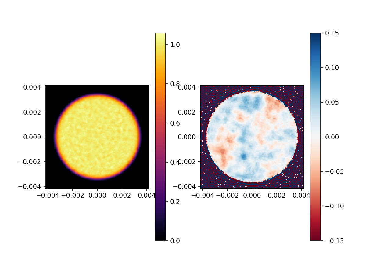
Add amplitude aberrations
Let’s now add ampitude aberrations. These are introduced in a telescope
by, for example, coating variations and surface errors on optical
elementsin a non-conjugate pupil. We will use the latter as an example
here and use the built-in SurfaceAberrationAtDistance class, which
performs a Fresnel propagation to the supplied distance, applies the
surface aberration, and performs a Fresnel propagation back to the
original plane.
Because the SurfaceAberrationAtDistance uses a Fresnel propagation,
we need to switch to physical units. We redefine our pupil grid and all
optical elements:
aberration_distance = 100e-3 # m

aberration_at_distance = SurfaceAberrationAtDistance(aberration, aberration_distance)

aberrated_pupil = aberration_at_distance(Wavefront(aperture, wavelength))

plt.subplot(1,2,1)
imshow_field(aberrated_pupil.intensity, cmap='inferno')
plt.colorbar()
plt.subplot(1,2,2)
imshow_field(aberrated_pupil.phase, cmap='RdBu', vmin=-0.15, vmax=0.15)
plt.colorbar()
plt.show()
def get_image(actuators=None, include_aberration=True):
    if actuators is not None:
        deformable_mirror.actuators = actuators

    wf = Wavefront(aperture, wavelength)
    if include_aberration:
        wf = aberration_at_distance(wf)

    img = prop(coronagraph(deformable_mirror(wf)))

    return img
jacobian = get_jacobian_matrix(get_image, dark_zone, len(influence_functions))

actuators, electric_fields, images = run_efc(get_image, dark_zone, len(influence_functions), jacobian)
Let’s plot this as an animation.
make_animation_1dm(actuators, electric_fields, images, dark_zone)
Now, the left side only reduces a tiny bit, as all amplitude aberrations are still in the system and we are using only a single deformable mirror for correction.
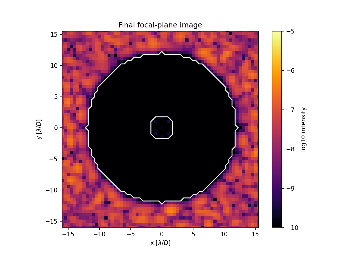
Adding a second deformable mirror
To correct the dark zone on both sides of the star with both phase and amplitude aberrations, we need to use two deformable mirrors, for example, one in the conjugate pupil, and one outside. Let’s add the deformable mirrors.
distance_between_dms = 200e-3 # m

dm1 = DeformableMirror(influence_functions)
dm2 = DeformableMirror(influence_functions)

prop_between_dms = FresnelPropagator(pupil_grid, distance_between_dms)

dark_zone_twosided = circular_aperture(2 * owa)(focal_grid)
dark_zone_twosided -= circular_aperture(2 * iwa)(focal_grid)
dark_zone_twosided = dark_zone_twosided.astype('bool')
def get_image(actuators=None, include_aberration=True):
    if actuators is not None:
        dm1.actuators = actuators[:len(influence_functions)]
        dm2.actuators = actuators[len(influence_functions):]

    wf = Wavefront(aperture, wavelength)
    if include_aberration:
        wf = aberration_at_distance(wf)

    wf_post_dms = prop_between_dms.backward(dm2(prop_between_dms.forward(dm1(wf))))
    img = prop(coronagraph(wf_post_dms))

    return img
jacobian = get_jacobian_matrix(get_image, dark_zone_twosided, 2 * len(influence_functions))

actuators, electric_fields, images = run_efc(get_image, dark_zone_twosided, 2 * len(influence_functions), jacobian)
Let’s plot this as an animation. As we’re now using multiple deformable mirrors, we need to create a new plot function.
plt.title('Final focal-plane image')
imshow_field(np.log10(images[-1] / img_ref.max()), grid_units=spatial_resolution, cmap='inferno', vmin=-10, vmax=-5)
plt.colorbar().set_label('log10 intensity')
contour_field(dark_zone_twosided, grid_units=spatial_resolution, levels=[0.5], colors='white')
plt.xlabel('x [$\lambda/D$]')
plt.ylabel('y [$\lambda/D$]')
plt.show()
def make_animation_2dm(actuators, electric_fields, images, dark_zone):
    anim = FFMpegWriter('video.mp4', framerate=5)

    num_iterations = len(actuators)
    average_contrast = [np.mean(image[dark_zone] / img_ref.max()) for image in images]

    electric_field_norm = mpl.colors.LogNorm(10**-5, 10**(-2.5), True)

    for i in range(num_iterations):
        dm1.actuators = actuators[i][:len(influence_functions)]
        dm2.actuators = actuators[i][len(influence_functions):]

        plt.clf()

        plt.subplot(2, 2, 1)
        plt.title('Electric field')
        electric_field = electric_fields[i] / np.sqrt(img_ref.max())
        imshow_field(electric_field, norm=electric_field_norm, grid_units=spatial_resolution)
        contour_field(dark_zone, grid_units=spatial_resolution, levels=[0.5], colors='white')

        plt.subplot(2, 2, 2)
        plt.title('Intensity image')
        imshow_field(np.log10(images[i] / img_ref.max()), grid_units=spatial_resolution, cmap='inferno', vmin=-10, vmax=-5)
        plt.colorbar()
        contour_field(dark_zone, grid_units=spatial_resolution, levels=[0.5], colors='white')

        plt.subplot(2, 3, 4)
        plt.title('DM1 surface in nm')
        imshow_field(dm1.surface * 1e9, grid_units=pupil_diameter, mask=aperture, cmap='RdBu', vmin=-5, vmax=5)
        plt.colorbar()

        plt.subplot(2, 3, 5)
        plt.title('DM2 surface in nm')
        imshow_field(dm2.surface * 1e9, grid_units=pupil_diameter, mask=aperture, cmap='RdBu', vmin=-5, vmax=5)
        plt.colorbar()

        plt.subplot(2, 3, 6)
        plt.title('Average contrast')
        plt.plot(range(i), average_contrast[:i], 'o-')
        plt.xlim(0, num_iterations)
        plt.yscale('log')
        plt.ylim(1e-11, 1e-5)
        plt.grid(color='0.5')

        plt.suptitle('Iteration %d / %d' % (i + 1, num_iterations), fontsize='x-large')

        anim.add_frame()

    plt.close()
    anim.close()

    return anim

make_animation_2dm(actuators, electric_fields, images, dark_zone_twosided)
os.remove('video.mp4')