Introduction to polarization
We will introduce how polarization is simulated in HCIPy, both for full and partially polarized light. We will show which polarization optical elements are implemented and how these are used.
We’ll start by implementing the required packages and set up a circular pupil.
from hcipy import *
import numpy as np
import matplotlib.pyplot as plt

pupil_grid = make_pupil_grid(256)

aperture = make_magellan_aperture(True)(pupil_grid)
Types of polarized Wavefronts
HCIPy supports three different types of wavefronts, which indicate different types of polarization. These are:
Scalar wavefronts
Fully polarized wavefronts
Partially polarized wavefronts
Each of these different types of wavefronts are implemented in a
Wavefront object. There are a number of ways to get the polarization
state of the Wavefront. These include (components of) the Stokes
vector, the degree of linear/circular polarization, etc… The different
types of wavefronts are distinguished by the tensor shape of the
electric_field that is in the Wavefront.
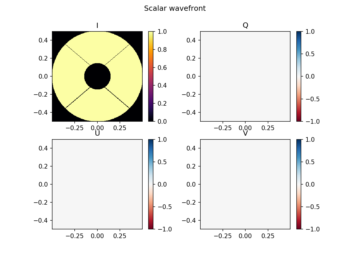
When you are not using polarization, you are most likely mostly using
scalar wavefronts. These contain a scalar electric_field.
scalar_wavefront = Wavefront(aperture)
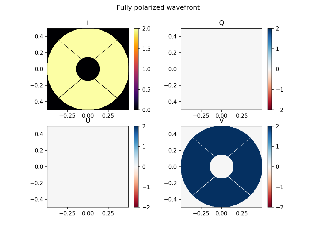
Fully polarized wavefronts use Jones vectors as their electric fields.
This means that the electric field will be a vector Field with two
components:
.
jones_vector = Field([aperture, 1j * aperture], pupil_grid)

fully_polarized_wavefront = Wavefront(jones_vector)
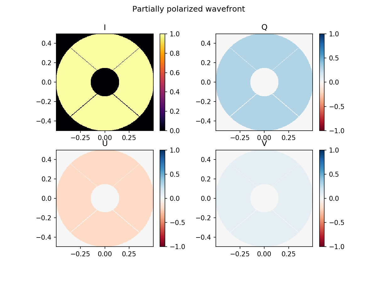
Partially polarized wavefronts use Jones matrices as their electric
fields. The electric field will be a 2x2 tensor Field:
These Jones matrices describe the change in polarization state and also phase and amplitude, from the initial wavefront to the current wavefront. The polarization state itself is set as the Stokes vector of the initial wavefront. Note that, in this way, HCIPy doesn’t support spatially varying degrees of polarization.
While you can create a full Jones matrix Field and pass that as the
electric field argument of the Wavefront, like this:
jones_matrix = Field([[aperture, aperture * 1j], [aperture * 1j, aperture]], pupil_grid)
stokes_vector = [1, 0.3, -0.2, 0.1]

partially_polarized_wavefront = Wavefront(jones_matrix, input_stokes_vector=stokes_vector)
in most cases, we are trying to create a Wavefront at the start of
our optical system. In this case we can pass a scalar electric field,
but add an input Stokes vector as well. This creates a Jones matrix
Field which has for each pixel an identity matrix multiplied by the
scalar wavefront at that position. For example, creating a partially
polarized Wavefront at our telescope pupil, we would do:
stokes_vector = [1, 0.3, -0.2, 0.1]

partially_polarized_wavefront = Wavefront(aperture, input_stokes_vector=stokes_vector)
Polarization attributes of Wavefronts
We can look at the Stokes components of the wavefront, and show them:
def imshow_stokes_vector(wavefront):
    I_max = wavefront.I.max()

    plt.subplot(2, 2, 1)
    plt.title('I')
    imshow_field(wavefront.I, cmap='inferno')
    plt.colorbar()

    plt.subplot(2, 2, 2)
    plt.title('Q')
    imshow_field(wavefront.Q, cmap='RdBu', vmin=-I_max, vmax=I_max)
    plt.colorbar()

    plt.subplot(2, 2, 3)
    plt.title('U')
    imshow_field(wavefront.U, cmap='RdBu', vmin=-I_max, vmax=I_max)
    plt.colorbar()

    plt.subplot(2, 2, 4)
    plt.title('V')
    imshow_field(wavefront.V, cmap='RdBu', vmin=-I_max, vmax=I_max)
    plt.colorbar()
plt.suptitle('Scalar wavefront')
imshow_stokes_vector(scalar_wavefront)
plt.show()
plt.suptitle('Fully polarized wavefront')
imshow_stokes_vector(fully_polarized_wavefront)
plt.show()
plt.suptitle('Partially polarized wavefront')
imshow_stokes_vector(partially_polarized_wavefront)
plt.show()
We can also show the polarization fraction:
fig, axes = plt.subplots(nrows=1, ncols=3)

axes[0].set_title('Scalar wavefront')
imshow_field(scalar_wavefront.degree_of_polarization, vmin=0, vmax=1, cmap='inferno', mask=aperture, ax=axes[0])

axes[1].set_title('Fully polarized wavefront')
imshow_field(fully_polarized_wavefront.degree_of_polarization, vmin=0, vmax=1, cmap='inferno', mask=aperture, ax=axes[1])

axes[2].set_title('Partially polarized wavefront')
imshow_field(partially_polarized_wavefront.degree_of_polarization, vmin=0, vmax=1, cmap='inferno', mask=aperture, ax=axes[2])

plt.colorbar(ax=axes.tolist(), orientation="horizontal")
/Users/epor/anaconda3/envs/hcipy-docs-v0.3.1/lib/python3.6/site-packages/hcipy/optics/wavefront.py:253: RuntimeWarning: invalid value encountered in true_divide
  return np.sqrt(self.Q**2 + self.U**2 + self.V**2) / self.I
<matplotlib.colorbar.Colorbar at 0x7fd6a8954550>
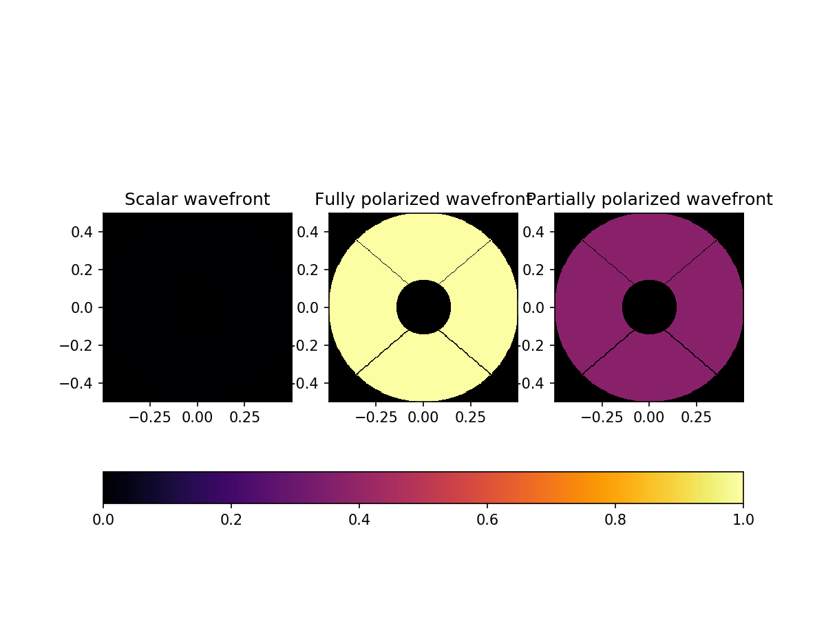
We can see that the scalar wavefront is considered an unpolarized wavefront, the fully polarized wavefront is 100% polarized, and the partially polarized wavefront permits a partial polarization fraction, which is exactly as we expected.
Optical propagation with polarized wavefronts
Optical propagations through optical elements with polarized wavefronts
are seamless. Take for example a FraunhoferPropagator propagation.
focal_grid = make_focal_grid(3, 8)
prop = FraunhoferPropagator(pupil_grid, focal_grid)

scalar_image = prop(scalar_wavefront)
fully_polarized_image = prop(fully_polarized_wavefront)
partially_polarized_image = prop(partially_polarized_wavefront)
plt.suptitle('Partially polarized wavefront')
imshow_stokes_vector(partially_polarized_image)
plt.show()
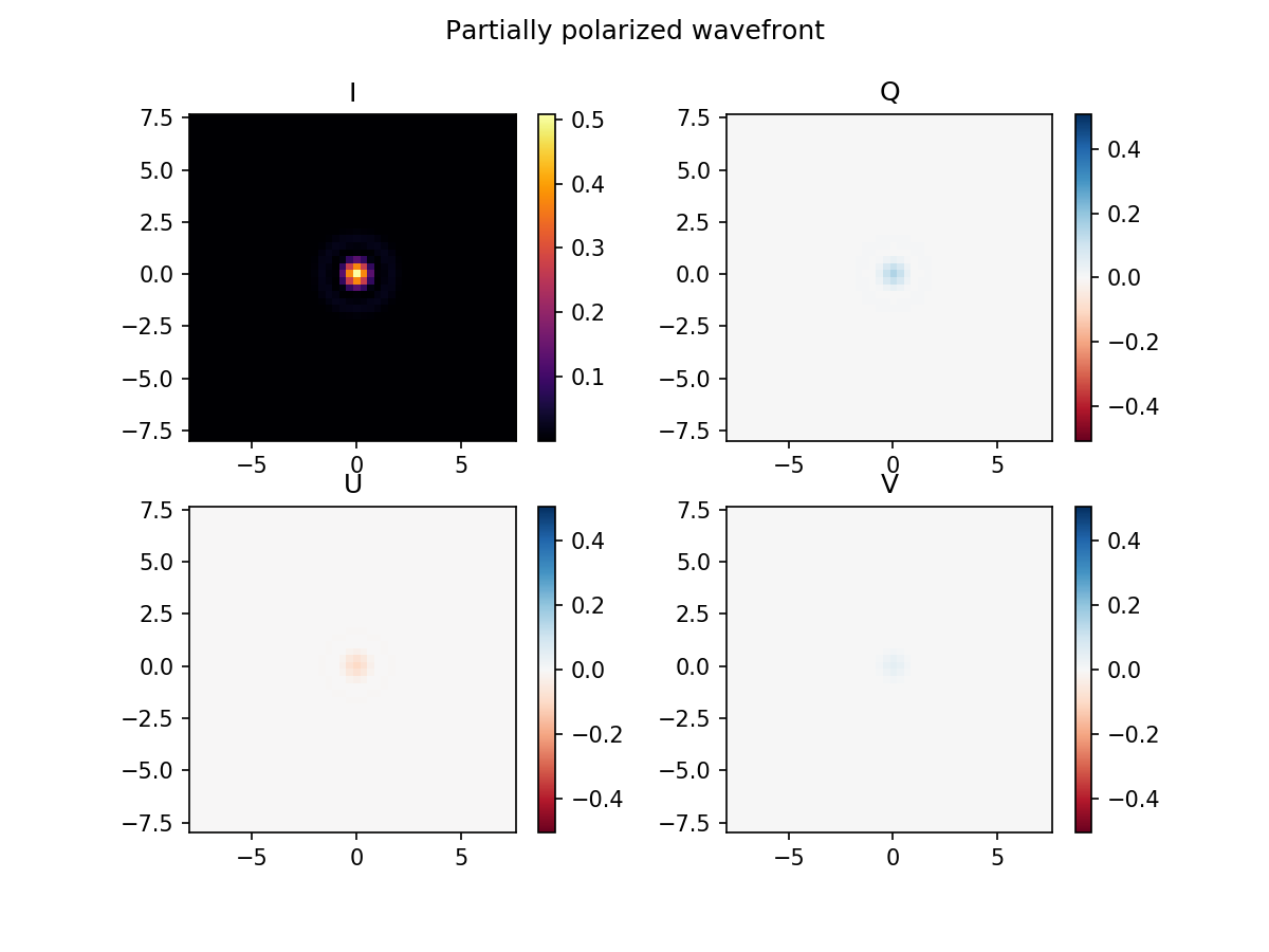
As the FraunhoferPropagator does not act differently depending on
the polarization of the incoming light, we see a normal Airy core which
has the same polarization state as we put in. Note that the call to the
propagator does not change depending on the type of the Wavefront
that we propagate through it. All calls look exactly the same. This
means that if we create a full optical system, consisting of many
optical elements in a row, that any Wavefront can be propgated
through, and we do not need to worry about having to rewrite the optical
system when we want to switch to (partially) polarized light.
HCIPy contains many polarization optical elements, such as half-wave plates, quarter-wave plates, general phase retarders, polarizers, polarizing beam splitters and more. Let’s simulate a high-contrast imaging scenario of an unpolarized star and a partially polarized planet next to it.
stokes_vector_planet = [1, 0.1, 0, 0]
contrast = 3e-4
angular_separation = 5 # lambda / D
num_photons_star = 1e9

wf_star = Wavefront(aperture)
wf_star.total_power = num_photons_star

e_planet = aperture * np.exp(2j * np.pi * pupil_grid.x * angular_separation)
wf_planet = Wavefront(e_planet, input_stokes_vector=stokes_vector_planet)
wf_planet.total_power = num_photons_star * contrast

# Calculate science image for the star and planet
science_image = prop(wf_star).power
science_image += prop(wf_planet).power

# Simulate photon noise
science_image = large_poisson(science_image)

imshow_field(np.log10(science_image / science_image.max() + 1e-20), vmin=-5, vmax=0)
plt.colorbar()
plt.show()
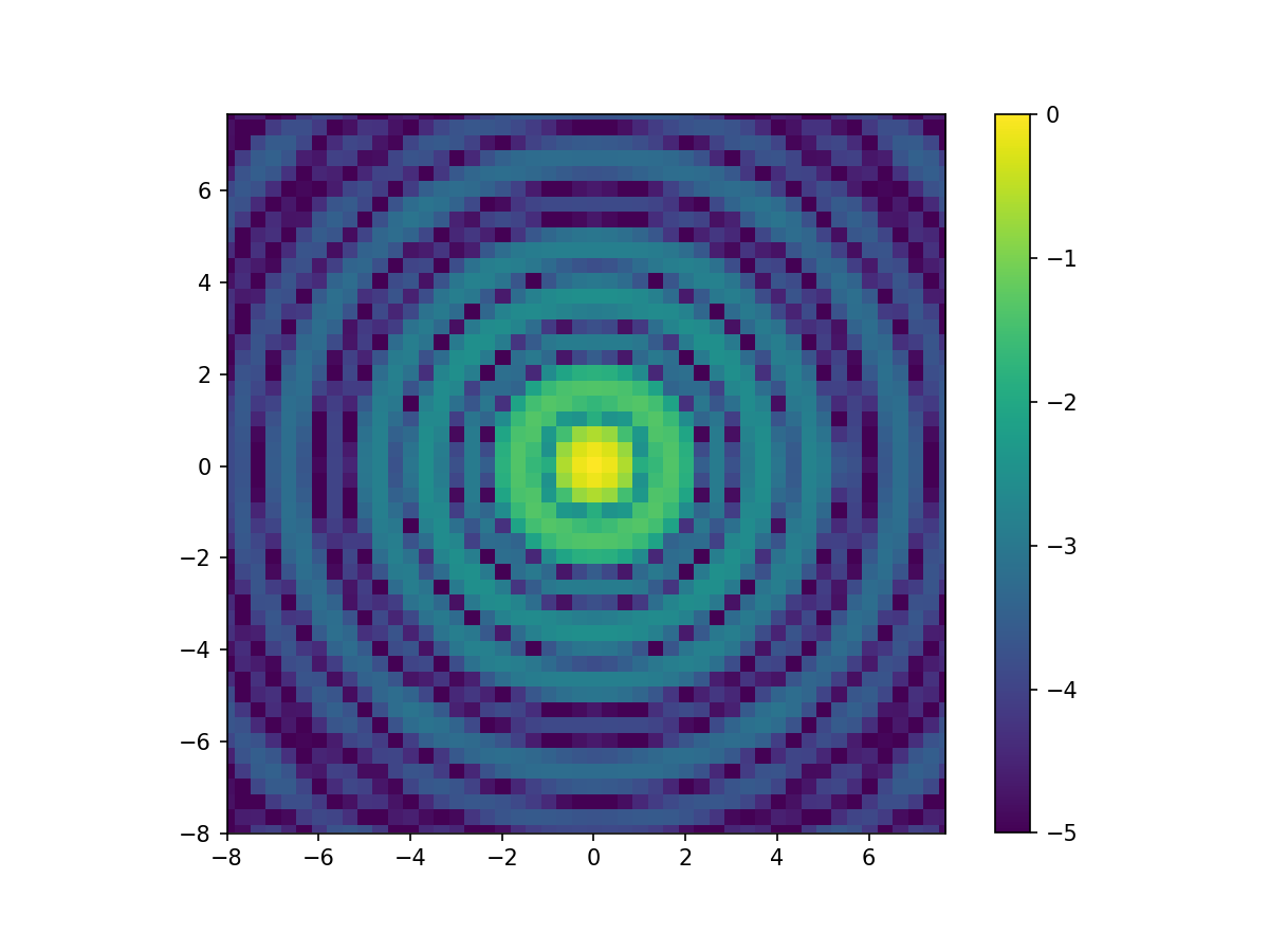
In this intensity image it is impossible to see the planet. It is completely buried below the light from the star. We need to look at a polarized light image. The simplest way, in fact to the point of oversimplification, is to split the light with a linear polarizing beam splitter and look at the difference between the two images. If the planet is polarized, it will show up in the difference image.
Let’s create a linear polarizing beam splitter object, and propagate the
star and planet Wavefronts through it. This creates two
wavefronts, one for each port of the beam splitter. The image for each
port is calculated.
pbs = LinearPolarizingBeamSplitter(0)

img_star_1, img_star_2 = pbs(prop(wf_star))
img_planet_1, img_planet_2 = pbs(prop(wf_planet))

science_image_1 = img_star_1.power + img_planet_1.power
science_image_2 = img_star_2.power + img_planet_2.power

science_image_1 = large_poisson(science_image_1)
science_image_2 = large_poisson(science_image_2)
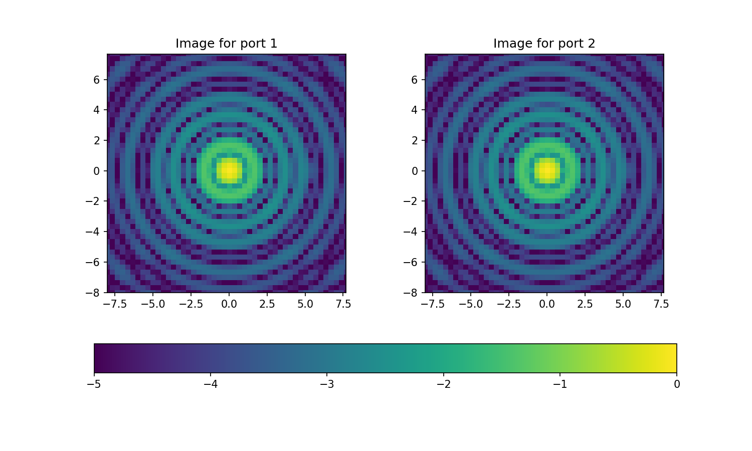
We can now show these two images and their difference.
fig, axes = plt.subplots(figsize=(10, 6), nrows=1, ncols=2)

axes[0].set_title('Image for port 1')
imshow_field(np.log10(science_image_1 / science_image_1.max() + 1e-20), vmin=-5, vmax=0, ax=axes[0])

axes[1].set_title('Image for port 2')
imshow_field(np.log10(science_image_2 / science_image_2.max() + 1e-20), vmin=-5, vmax=0, ax=axes[1])

plt.colorbar(ax=axes.tolist(), orientation="horizontal")
plt.show()

plt.title('Difference')
imshow_field((science_image_1 - science_image_2) / science_image_1.max(), cmap='RdBu', vmin=-1e-4, vmax=1e-4)
plt.annotate('planet', xy=(5, -1), xytext=(3, -7), arrowprops={'arrowstyle': '-|>'})
plt.colorbar()
plt.show()
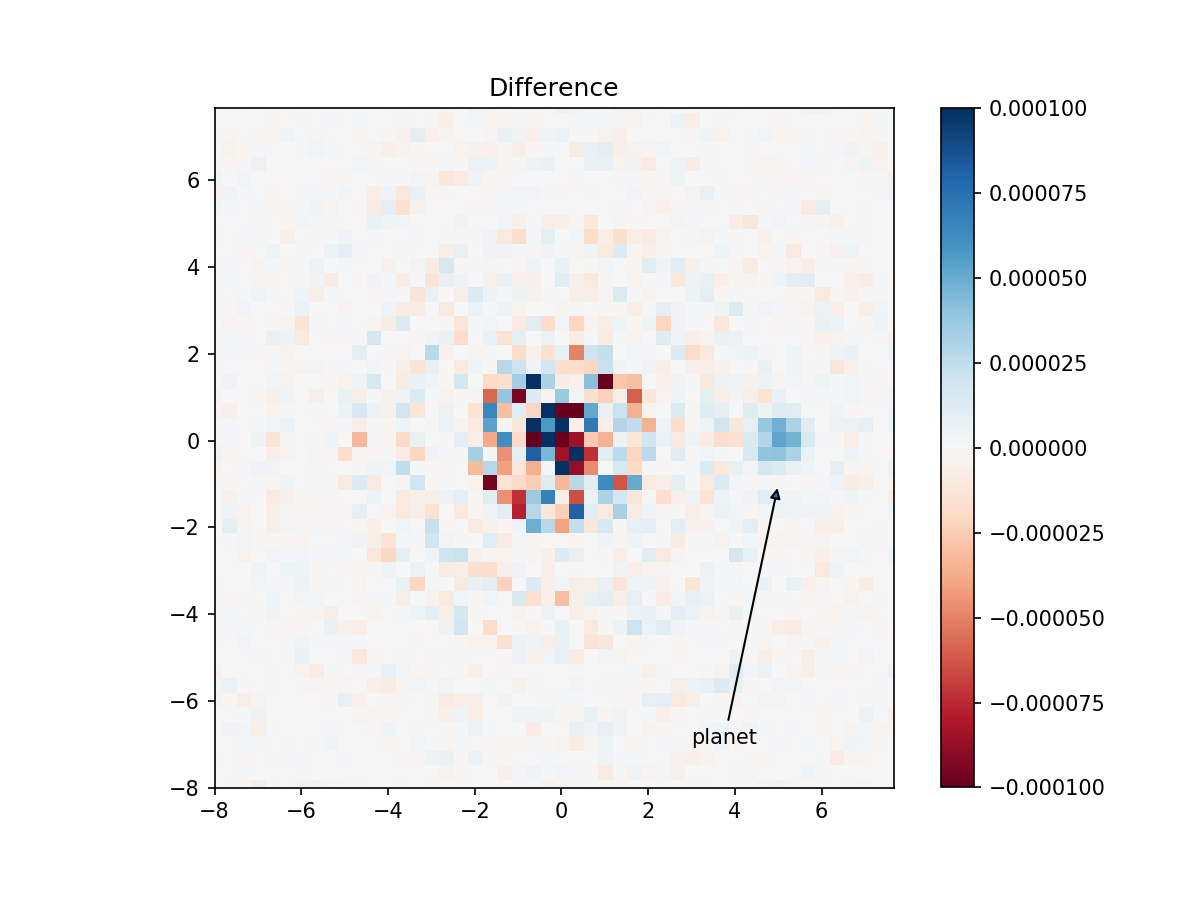
In the difference image we can clearly see the planet light up. It has a contrast of \(3\times10^{-5}\), which is partly due to the contrast of the planet (\(3\times10^{-4}\)) and the degree of polarization of the planet (10%). While this is clearly a simplified example (it can only detect the Q-component of the planet), it shows the simplicity and power of HCIPy for propagating polarized light.
This introduction falls short of the many other optical elements that act on polarization. Other tutorials showcase some more of these optical elements. These include, but are not limited to, a simple polarimeter and imaging with a vector apodizing phase plate coronagraph.