Near and far-field diffraction
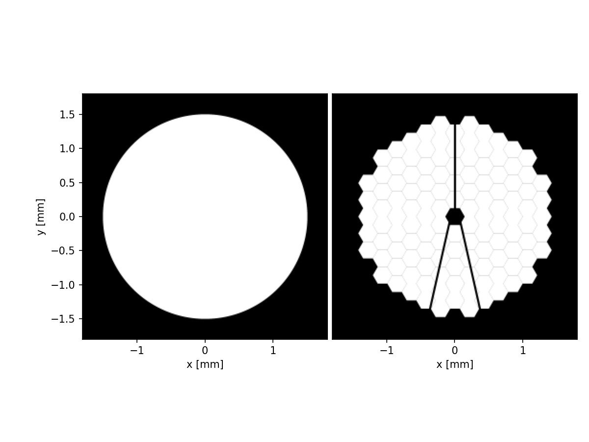
We will demonstrate the near and far-field propagators in HCIPy. We’ll use both a circular aperture and the LUVOIR-A telescope pupil as example pupils.
We first start by importing the relevant python modules.
from hcipy import *
import numpy as np
import matplotlib.pyplot as plt
%matplotlib inline
To make life simpler later on, we define a function to nicely show two fields side-to-side, with a nice spacing, titles and axes labels.
def double_plot(a, b, title='', xlabel='', ylabel='', **kwargs):
'''A function to nicely show two fields side-to-side.
'''
fig, axes = plt.subplots(1, 2, gridspec_kw={'left': 0.14, 'right': 0.98, 'top': 0.95, 'bottom': 0.07, 'wspace': 0.02})
fig.suptitle(title)
imshow_field(a, **kwargs, ax=axes[0])
imshow_field(b, **kwargs, ax=axes[1])
axes[1].yaxis.set_ticks([])
axes[0].set_xlabel(xlabel)
axes[1].set_xlabel(xlabel)
axes[0].set_ylabel(ylabel)
return fig
Now we can create the pupils. Each pupil will have the same diameter of 3mm, and we’ll use a wavelength of 500nm. Each pupil is evaluated with supersampling, meaning that the value at each pixel will be the average of, in our case, 8x8=64 subpixels. We’ll use 256 pixels across and enlarge the pupil plane slightly to be able to see the details in the near-field diffraction just outside of the pupil.
pupil_diameter = 3e-3 # meter
wavelength = 500e-9 # meter
pupil_grid = make_pupil_grid(256, 1.2 * pupil_diameter)
aperture_circ = evaluate_supersampled(circular_aperture(pupil_diameter), pupil_grid, 8)
aperture_luvoir = evaluate_supersampled(make_luvoir_a_aperture(True), pupil_grid.scaled(1 / pupil_diameter), 8)
aperture_luvoir.grid = pupil_grid
wf_circ = Wavefront(aperture_circ, wavelength)
wf_luvoir = Wavefront(aperture_luvoir, wavelength)
/var/folders/_3/tqcb9bj94nd9xz_wqt4_3g2h0000gn/T/ipykernel_26688/3917442576.py:5: DeprecationWarning: circular_aperture is deprecated. Its new name is make_circular_aperture.
aperture_circ = evaluate_supersampled(circular_aperture(pupil_diameter), pupil_grid, 8)
And plotting both apertures next to each other:
double_plot(aperture_circ, aperture_luvoir,
xlabel='x [mm]', ylabel='y [mm]',
grid_units=1e-3, cmap='gray')
plt.show()
Near-field propagation
Near-field diffraction is used for propagation of waves in the near
field. In HCIPy we have currently two propagators for simulating
near-field diffraction. We will only use the
:class:FresnelPropagator. This propagator uses the paraxial Fresnel
approximation to propagate a :class:Wavefront. We can create the
propagator as follows:
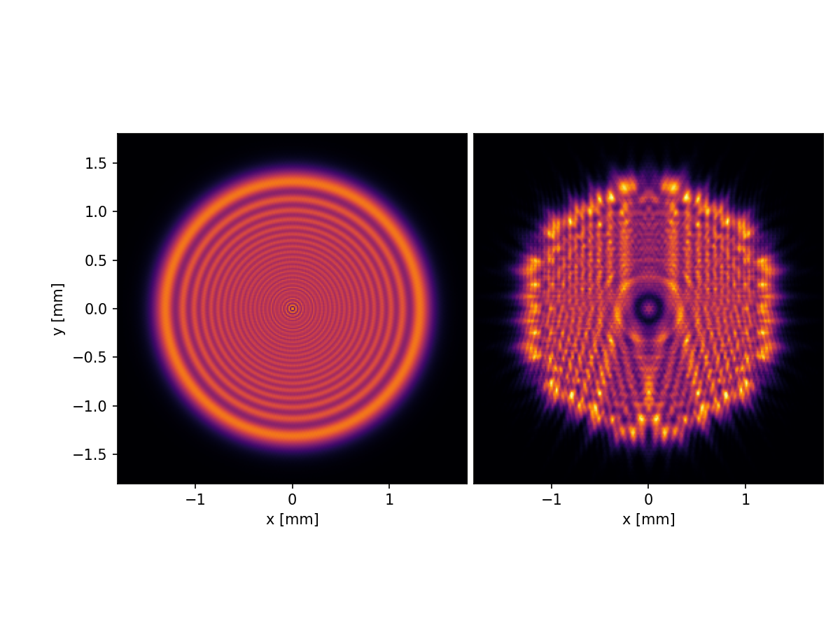
propagation_distance = 0.1 # meter
fresnel = FresnelPropagator(pupil_grid, propagation_distance)
Afterwards we can simply propagate a wavefront through the created
Fresnel propagator by calling it with the wavefront. Alternatively, you
can also call the propagator.forward() or propagator.backward()
functions for forward and backward propagation.
img_circ = fresnel(wf_circ)
img_luvoir = fresnel(wf_luvoir)
And plotting the result.
double_plot(img_circ.intensity, img_luvoir.intensity,
xlabel='x [mm]', ylabel='y [mm]',
vmax=2, cmap='inferno', grid_units=1e-3)
plt.show()
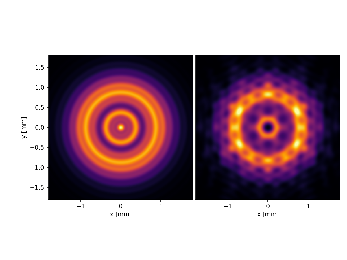
We can modify the distance by changing the distance parameter of the
propagator. Alternatively, we can create a new
:class:FresnelPropagator object using the new distance.
fresnel.distance = 1 # meter
img_circ = fresnel(wf_circ)
img_luvoir = fresnel(wf_luvoir)
double_plot(img_circ.intensity, img_luvoir.intensity,
xlabel='x [mm]', ylabel='y [mm]',
vmax=2, cmap='inferno', grid_units=1e-3)
plt.show()
It’s always nice to see the full transition from near-field to far-field diffraction. We’ll make an animation to slowly transition from 0 to 20 meters.
def easing(start, end, n):
x = np.linspace(0, 1, n)
y = np.where(x < 0.5, 4 * x**3, 1 - 4 * (1 - x)**3)
return y * (end - start) + start
# Setting up the propagation distances in the animation
n = 35
propagation_distances = np.concatenate([easing(0, 0.1, n),
easing(0.1, 1, n),
easing(1, 5, n),
easing(5, 20, n),
easing(20, 0, 2 * n)])
# Starting the animation object to write to an mp4 file.
anim = FFMpegWriter('near_field.mp4', framerate=11)
for propagation_distance in propagation_distances:
# Set the propagation distance
fresnel.distance = propagation_distance
# Propagate both wavefronts
img_circ = fresnel(wf_circ)
img_luvoir = fresnel(wf_luvoir)
# Plotting the current frame of the animation.
double_plot(img_circ.intensity, img_luvoir.intensity,
title='Distance: %.3f meter' % propagation_distance,
xlabel='x [mm]', ylabel='y [mm]',
vmax=2, cmap='inferno', grid_units=1e-3)
# Adding the frame to the mp4 file and closing the created figure.
anim.add_frame()
plt.close()
anim.close()
anim
Far-field propagation
Far-field diffraction uses the Fraunhofer approximation to propagate
waves. In high-contrast imaging, we often use lenses or mirrors with a
specified focal length to focus the light from a pupil plane into a
focal plane. In HCIPy we can do the same thing with a
:class:FraunhoferPropagator object. This propagator propagates from
a pupil to a focal plane with a perfect lens.
First we have to define our focal length and the sampling of the focal plane that we want to get out.
focal_length = 0.5 # meter
spatial_resolution = focal_length / pupil_diameter * wavelength
focal_grid = make_focal_grid(8, 12, spatial_resolution=spatial_resolution)
Then we can create our :class:FraunhoferPropagator object and pass
the pupil and focal grids, and the focal length of its perfect lens.
fraunhofer = FraunhoferPropagator(pupil_grid, focal_grid, focal_length=focal_length)
Then we can propagate our wavefronts and plot the resulting images as usual.
img_circ = fraunhofer(wf_circ)
img_luvoir = fraunhofer(wf_luvoir)
double_plot(img_circ.power, img_luvoir.power,
xlabel='x [um]', ylabel='y [um]',
cmap='inferno', grid_units=1e-6)
plt.show()
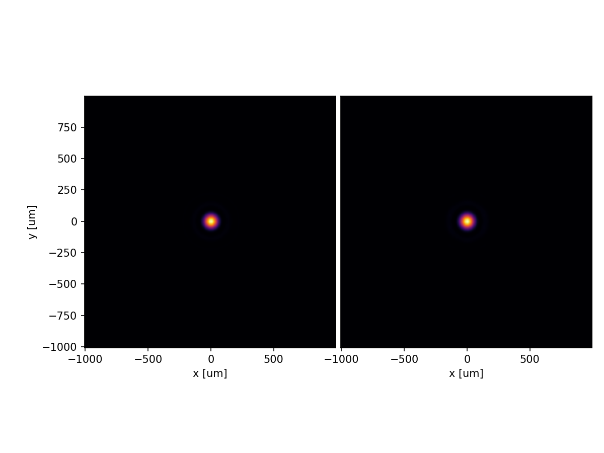
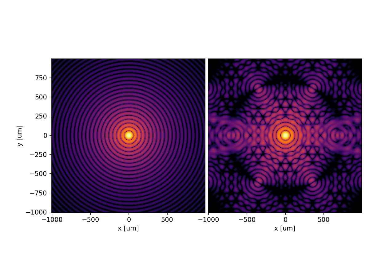
Due to the contrast in the focal plane, there is barely any difference between the two telescope pupils. We can make this clearer by showing the images on a logarithmic scale.
double_plot(np.log10(img_circ.power / img_circ.power.max()), np.log10(img_luvoir.power / img_luvoir.power.max()),
xlabel='x [um]', ylabel='y [um]',
vmin=-6, cmap='inferno', grid_units=1e-6)
plt.show()
Changing the focal length is as simple as modifying the focal_length
parameter, or we can create a new propagator with the new focal length.
The PSF shrinks with a smaller focal length of 30cm.
fraunhofer.focal_length = 0.3 # m
img_circ = fraunhofer(wf_circ)
img_luvoir = fraunhofer(wf_luvoir)
double_plot(np.log10(img_circ.power / img_circ.power.max()), np.log10(img_luvoir.power / img_luvoir.power.max()),
xlabel='x [um]', ylabel='y [um]',
vmin=-6, cmap='inferno', grid_units=1e-6)
plt.show()
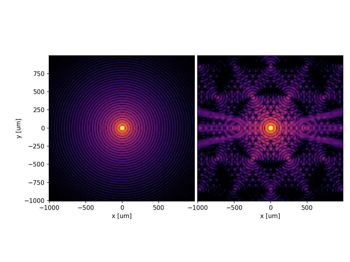
Changing the wavelength is done by changing wavelength parameter of the
:class:Wavefront objects that are passed to the propagators. With a
smaller wavelength of 350nm, our PSFs will shrink even more.
wf_circ.wavelength = 350e-9 # meter
wf_luvoir.wavelength = 350e-9 # meter
img_circ = fraunhofer(wf_circ)
img_luvoir = fraunhofer(wf_luvoir)
double_plot(np.log10(img_circ.power / img_circ.power.max()), np.log10(img_luvoir.power / img_luvoir.power.max()),
xlabel='x [um]', ylabel='y [um]',
vmin=-6, cmap='inferno', grid_units=1e-6)
plt.show()
Of course, we can easily create an animation of the PSF changes with wavelength.
fraunhofer.focal_length = 0.5 # meter
n = 50
wavelength_max = 700e-9
wavelength_min = 350e-9
wavelengths = np.concatenate([easing(wavelength_min, wavelength_max, n),
easing(wavelength_max, wavelength_min, n)])
anim = FFMpegWriter('far_field.mp4', framerate=15)
for wl in wavelengths:
wf_circ.wavelength = wl
wf_luvoir.wavelength = wl
img_circ = fraunhofer(wf_circ)
img_luvoir = fraunhofer(wf_luvoir)
double_plot(np.log10(img_circ.power / img_circ.power.max()), np.log10(img_luvoir.power / img_luvoir.power.max()),
title='Wavelength: %d nm' % (wl * 1e9),
xlabel='x [um]', ylabel='y [um]',
vmin=-6, cmap='inferno', grid_units=1e-6)
anim.add_frame()
plt.close()
anim.close()
anim
# Cleanup created files
import os
os.remove('near_field.mp4')
os.remove('far_field.mp4')