Telescope pupils and Grids

We will introduce the core elements in HCIPy (Grids and Fields) and will generate telescope pupils for all telescopes included in HCIPy.

import numpy as np
import matplotlib.pyplot as plt

from hcipy import *

Let’s create a VLT (Very Large Telescope) pupil. We can do this using the make_vlt_aperture() function:

vlt_aperture = make_vlt_aperture()

print(type(vlt_aperture))

<class 'function'>

We can see however that this does not return an image of the VLT pupil, but rather a Python function object. This function contains only the geometry of the VLT pupil itself, rather than an image of the pupil on a certain sampling. To create an image out of this function, we need to call it with a sampling that tells us where each pixel in the image is located. HCIPy uses a Grid for this. Let’s create one:

grid = make_pupil_grid(128, diameter=10)

print(type(grid))
print(type(grid.coords))

<class 'hcipy.field.cartesian_grid.CartesianGrid'>
<class 'hcipy.field.coordinates.RegularCoords'>

The function make_pupil_grid() is a convenience function to create a uniform sampling with Cartesian (x/y) coordinates. The diameter argument tells the function what the total extent of the sampling needs to be.

We can see that the function returned a CartesianGrid object, which indicates that its coordinates are on a Cartesian coordinate system. There are a few coordinate systems in HCIPy, most notably CartesianGrid and PolarGrid for Cartesian and polar coordinate systems respectively.

The raw numbers themselves that indicate where the sampling points are located, are stored in the Grid.coords attribute. We can see that make_pupil_grid() made a RegularCoords object for us, which indicates that our coordinates are regularly spaced in all axes. That is, the distance between points is constant.

To show the x and y sample points of this grid, we can simply access the CartesianGrid.x and CartesianGrid.y attributes of our grid:

print('x:', grid.x)
print('y:', grid.y)

x: [-4.9609375 -4.8828125 -4.8046875 ...  4.8046875  4.8828125  4.9609375]
y: [-4.9609375 -4.9609375 -4.9609375 ...  4.9609375  4.9609375  4.9609375]

Another useful attribute of a Grid is Grid.points. This stores a list of (x, y) values in a list, which makes it easy to get the coordinates for individual points in the grid:

print('x[100]:', grid.x[100])
print('y[100]:', grid.y[100])
print('(x, y):', grid.points[100])

x[100]: 2.8515625
y[100]: -4.9609375
(x, y): [ 2.8515625 -4.9609375]

Let’s see all these points in a plot:

plt.plot(grid.x, grid.y, '.')
plt.gca().set_aspect(1)
plt.xlabel('x [m]')
plt.ylabel('y [m]')
plt.show()

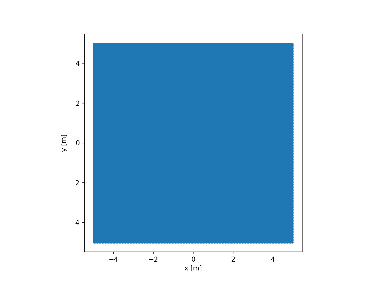
That’s a lot of points. Let’s zoom in on one of the corners to see what’s actually happening.

plt.plot(grid.x, grid.y, '.')
plt.gca().set_aspect(1)
plt.xlabel('x [m]')
plt.ylabel('y [m]')
plt.xlim(4, 5.2)
plt.ylim(4, 5.2)
plt.show()

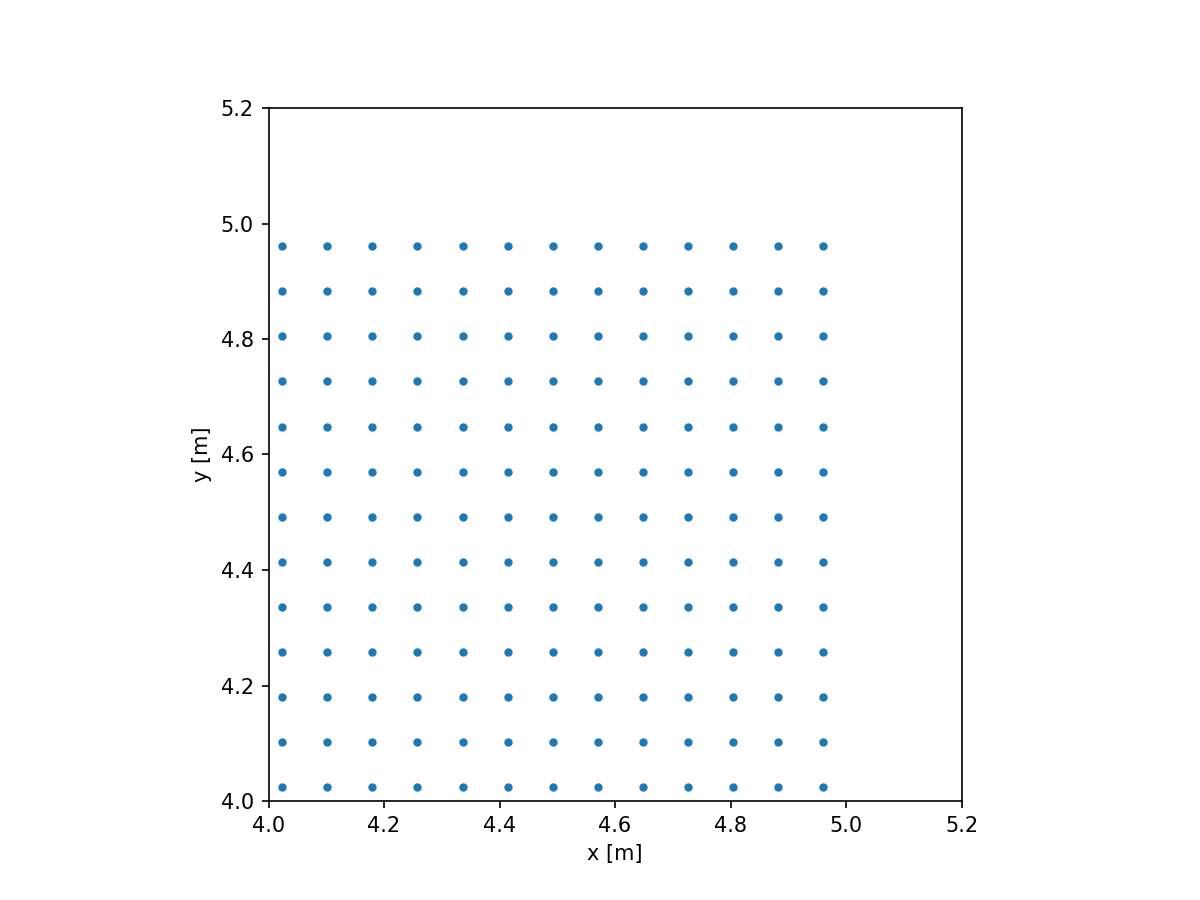
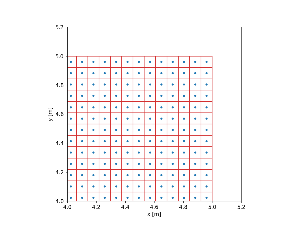
Note that the points do not extend all the way to (5, 5). While the pixels themselves do extend to the full extent, the centers of these pixels do not. We can make this more clear by drawing a rectangle around each point.

plt.plot(grid.x, grid.y, '.')
plt.gca().set_aspect(1)
plt.xlabel('x [m]')
plt.ylabel('y [m]')
plt.xlim(4, 5.2)
plt.ylim(4, 5.2)

for p in grid.points:
    rect = plt.Rectangle(p - grid.delta / 2, *grid.delta, linewidth=1, edgecolor=colors.red, facecolor='none')
    plt.gca().add_patch(rect)

plt.show()

Let’s get back to the aperture and make an image out of it by evaluation:

aperture = vlt_aperture(grid)

print(type(aperture))

<class 'hcipy.field.field.Field'>

So, the resulting object still isn’t a Numpy array, but a Field instead. In HCIPy, a Field object combines a Numpy array and a Grid:

print('The grid of aperture:', aperture.grid)

The grid of aperture: CartesianGrid(RegularCoords)

We can now show this field with the imshow_field() function. This function takes into account the grid on which the field is defined and uses it to set the right axes and scaling of the image.

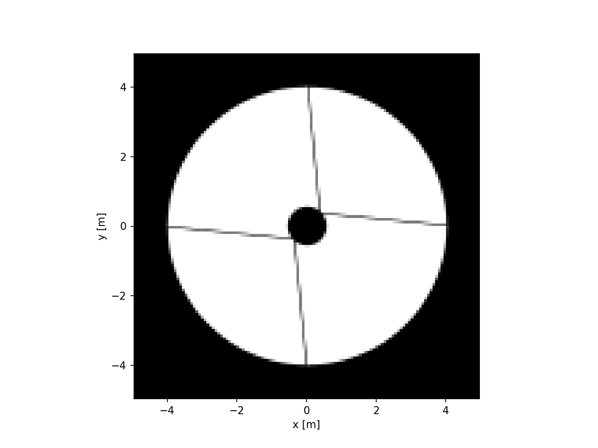
imshow_field(aperture, cmap='gray', interpolation='nearest')
plt.xlabel('x [m]')
plt.ylabel('y [m]')
plt.show()

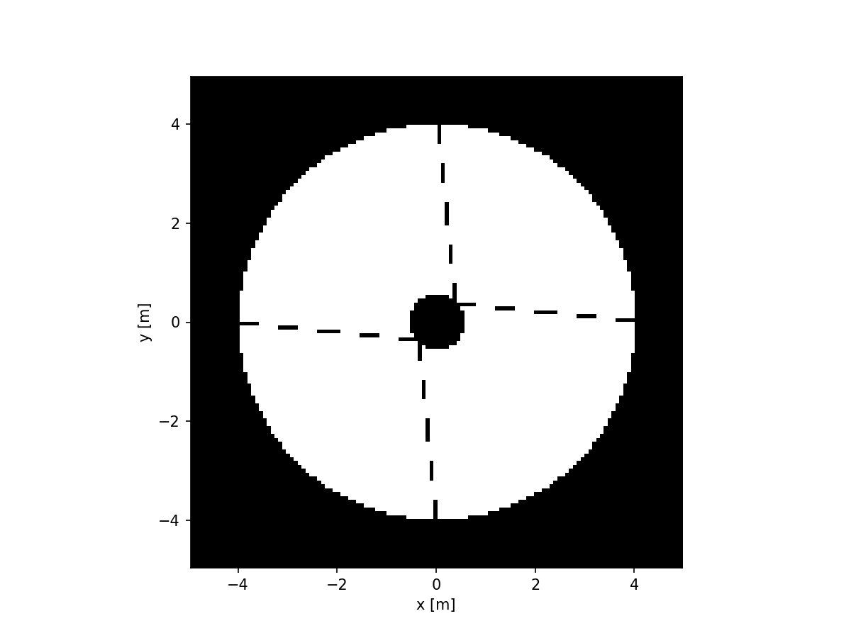
Note that the extent of this image is indeed the 10 meters that we specified when we first made this grid.

We can also see that the secondary support structure (or spider) is dashed instead of solid. This is due to pixellation. The underlying aperture is either zero or one, so if we evaluate it, the result is gonna be one of those values. Let’s zoom into the spider a bit and overlay the positions of the pixels:

imshow_field(aperture, cmap='gray', interpolation='nearest')
plt.plot(grid.x, grid.y, '.')
plt.xlabel('x [m]')
plt.ylabel('y [m]')
plt.xlim(2.5, 4.5)
plt.ylim(-0.85, 0.85)
plt.show()

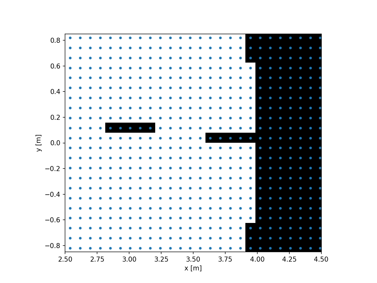
Here we can clearly see that happening. We can avoid this by increasing our sampling. Instead of creating a new pupil grid, now with 256 pixels across, let’s do something more interesting. Let’s supersample the grid that we already have and re-evaluate the aperture on that new grid.

grid_double = make_supersampled_grid(grid, 2)
aperture_double = vlt_aperture(grid_double)

imshow_field(aperture_double, cmap='gray', interpolation='nearest')
plt.plot(grid_double.x, grid_double.y, '.')
plt.xlabel('x [m]')
plt.ylabel('y [m]')
plt.xlim(2.5, 4.5)
plt.ylim(-0.85, 0.85)
plt.show()

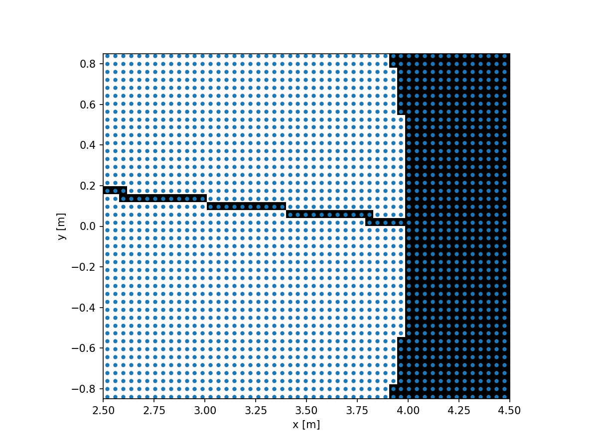
We can now see that we fully resolve the spider.

Sometimes using more pixels is not what we want, since this comes at the cost of computation time. Another way is to supersample the pixels themselves. That is, we increase the resolution by a certain factor (say 4x), so that each pixel is now composed of 4x4=16 subpixels. Then we evaluate our function on that high-resolution grid. Finally, we take the average of all subpixels to form our supersampled image.

Rather than doing this procedure manually, HCIPy has evaluate_supersampled() that does this for you, and in a slightly smarter way too.

aperture_supersampled = evaluate_supersampled(vlt_aperture, grid, 8)

imshow_field(aperture_supersampled, cmap='gray', interpolation='nearest')
plt.plot(grid.x, grid.y, '.')
plt.xlabel('x [m]')
plt.ylabel('y [m]')
plt.xlim(2.5, 4.5)
plt.ylim(-0.85, 0.85)
plt.show()

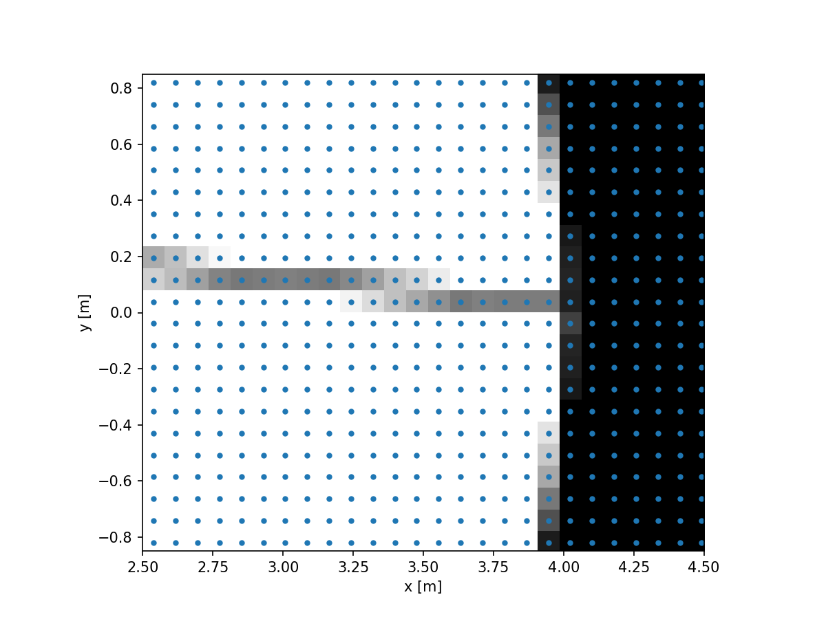
We can now see that we have a Field at the original resolution, but now with grayscale pixels. The full aperture now looks like:

imshow_field(aperture_supersampled, cmap='gray', interpolation='nearest')
plt.xlabel('x [m]')
plt.ylabel('y [m]')
plt.show()

which certainly looks more pleasingly by eye. This can improve on simulation fidelity without any additional computational cost (outside of the initial setup/calculation of the mask itself). This technique is used often for resolving small pupil features, such as thin spider vanes or the gaps between segments on segmented pupils.

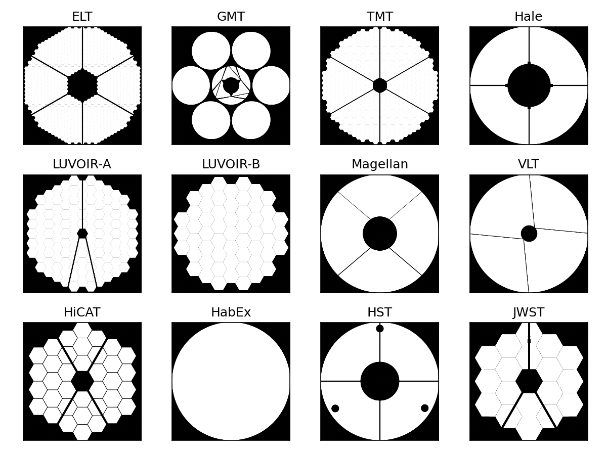
We are now ready to do the same for all telescope pupils implemented in HCIPy, and make a nice collage out of them. We’ll compute the images on a 512x512 grid, using 4x supersampling.

aperture_funcs = [
    ('ELT', make_elt_aperture),
    ('GMT', make_gmt_aperture),
    ('TMT', make_tmt_aperture),
    ('Hale', make_hale_aperture),
    ('LUVOIR-A', make_luvoir_a_aperture),
    ('LUVOIR-B', make_luvoir_b_aperture),
    ('Magellan', make_magellan_aperture),
    ('VLT', make_vlt_aperture),
    ('HiCAT', make_hicat_aperture),
    ('HabEx', make_habex_aperture),
    ('HST', make_hst_aperture),
    ('JWST', make_jwst_aperture),
]

pupil_grid = make_pupil_grid(512)

n_width = 4
n_height = 3

for i, (label, aperture) in enumerate(aperture_funcs):
    img = evaluate_supersampled(aperture(normalized=True), pupil_grid, 4)

    ax = plt.subplot(n_height, n_width, i + 1)
    ax.set_title(label)
    imshow_field(img, cmap='gray', interpolation='bilinear', ax=ax)
    ax.xaxis.set_ticks([])
    ax.yaxis.set_ticks([])

plt.tight_layout()
plt.show()